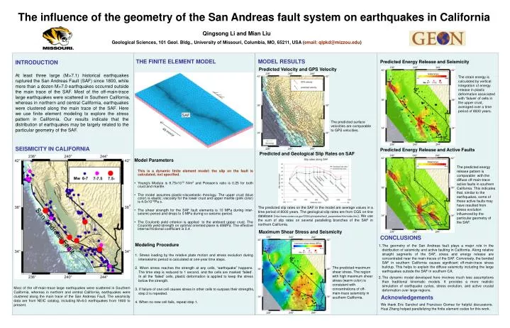
The influence of the geometry of the San Andreas fault system on earthquakes in California

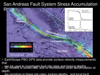
1. The influence of the geometry of the San Andreas fault system on earthquakes in California Qingsong Li and Mian Liu Geological Sciences, 101 Geol. Bldg., University of Missouri, Columbia, MO, 65211, USA (email: qlpkd@mizzou.edu) THE FINITE ELEMENT MODEL MODEL RESULTS INTRODUCTION Predicted Energy Release and Seismicity Predicted Velocity and GPS Velocity At least three large (M>7.1) historical earthquakes ruptured the San Andreas Fault (SAF) since 1800, while more than a dozen M>7.0 earthquakes occurred outside the main trace of the SAF. Most of the off-main-trace large earthquakes were scattered in Southern California, whereas in northern and central California, earthquakes were clustered along the main trace of the SAF. Here we use finite element modeling to explore the stress pattern in California. Our results indicate that the distribution of earthquakes may be largely related to the particular geometry of the SAF. The strain energy is calculated by vertical integration of energy release in plastic deformation associated with ‘failure’ of cells in the upper crust, averaged over a time period of 8000 years. The predicted surface velocities are comparable to GPS velocities. SEISMICITY IN CALIFORNIA Predicted Energy Release and Active Faults Predicted and Geological Slip Rates on SAF Model Parameters This is a dynamic finite element model: the slip on the fault is calculated, not specified. • Young’s Module is 8.75x1010 N/m2 and Poisson’s ratio is 0.25 for both crust and mantle. • The model assumes plastic-viscoelastic rheology. The upper crust (blue color) is elastic; viscosity for the lower crust and upper mantle (pink color) is 4.0x1019Pa s. • The shear strength for the SAF fault elements is 10 MPa during inter-seismic period and drops to 0 MPa during co-seismic period. • The Coulomb yield criterion is applied to the ambient upper crust. The Coulomb yield strength on optimal oriented plane is 45MPa. The effective internal frictional coefficient is 0.4 . The predicted energy release pattern is comparable with the diffuse off-main-trace active faults in southern California. This indicates that, similar to the earthquakes, some of these active faults may have resulted from stress evolution influenced by the particular geometry of the SAF. The predicted slip rates on the SAF in the model are average values in a time period of 8000 years. The geological slip rates are from CGS on-line database (http://www.consrv.ca.gov/CGS/rghm/psha/fault_parameters/htm/index.htm). We use the sum of slip rates on several paralleling branches of the SAF in northern California. Maximum Shear Stress and Seismicity CONCLUSIONS • Modeling Procedure • Stress loading by the relative plate motion and stress evolution during interseismic period is calculated at one-year time steps. • 2. When stress reaches the strength at any cells, “earthquake” happens. The time step is reduced to 1 second, and the cells are marked ‘failed’. In all the ‘failed’ cells, plastic deformation is applied to keep the stress below the strength. • 3. If failure of one cell causes stress in other cells to surpass their strengths, step 2 is repeated. • 4. When no new cell fails, repeat step 1. • The geometry of the San Andreas fault plays a major role in the distribution of seismicity and active faulting in California. Along relative straight segments of the SAF, stress and energy release are concentrated near the main-traces of the SAF. Conversely, the bended SAF in southern California causes significant off-main-trace stress buildup. This helps to explain the diffuse seismicity including the large earthquakes outside the SAF in southern CA. • The dynamic model developed here involves much less assumptions than traditional kinematic models. It provides a more realistic simulation of earthquake cycles, stress evolution, and active crustal deformation over large regions. The predicted maximum shear stress. The region with high maximum shear stress (warm color) is consistent with concentrations of off-main-trace seismicity in southern California. Most of the off-main-trace large earthquakes were scattered in Southern California, whereas in northern and central California, earthquakes were clustered along the main trace of the San Andreas Fault. The seismicity data are from NEIC catalog, including M>6.0 earthquakes from 1800 to present. Acknowledgements We thank Eric Sandvol and Francisco Gomez for helpful discussions. Huai Zhang helped parallelizing the finite element codes for this work.