Download
1 / 43
430 likes | 607 Views
Time Response. By Irfan Azhar. Transient Response. After the engineer obtains a mathematical representation of a subsystem, the subsystem is analyzed for its transient and steady-state responses to see if these characteristics yield the desired behavior.

E N D
Time Response By IrfanAzhar
Transient Response • After the engineer obtains a mathematical representation of a subsystem, the subsystem is analyzed for its transient and steady-state responses to see if these characteristics yield the desired behavior. • The output response of a system is the sum of two responses: the forced response and the natural response • Techniques like differential equations, inverse laplace transforms etc. can be used to evaluate output responses. • However, for Poles/Zeros analysis can also be used to analyze the system in less time.
Poles and Zeroes • When we get y(s) = P(s)/q(s) • The denominator polynomial q(s), when set equal to zero, is called the characteristic equation because the roots of this equation determine the character of the time response. • The roots of this characteristic equation are also called the poles of the system. • The roots of the numerator polynomial p(s) are called the zeros of the system • Poles and zeros are critical fre-quencies. At the poles, the function Y(s) becomes infinite. • At the zeros, the function becomes zero. • The complex frequency s-plane plot of the poles and zeros graphically portrays the character of the natural transient response of the system.
2nd order system • Did you notice!1st order systems did not have overshoot • A second order system is different • Changes in system parameters can change form of the response. • Could be like the 1st order system, or damped, or might have pure oscillations, depending on components. • We shall consider a system with 2 poles and no 0’s
General 2nd order system • Describe the system behavior without sketching the response! • Like we used time constants to describe the performance of 1 st order system, we will use damping ratio and natural frequency for the 2nd order system.
A system whose transient response goes through three cycles in a millisecond before reaching the steady state would have the same measure as a system that went through three cycles in a millennium before reaching the steady state. • The under damped curve in Figure 4.10 has an associated measure that defines its shape. This measure remains the same even if we change the time base from seconds to microseconds or to millennia. • A viable definition for this quantity is one that compares the exponential decay frequency of the envelope to the natural frequency.
Damping Ratio • The ratio is constant regardless of the time scale of the response. • The reciprocal, which is proportional to the ratio of the natural period to the exponential time constant, remains the same regardless of the time base.
Under Damped 2nd order System • Our first objective is to define transient specifications associated with underdamped responses. • Next we relate these specifications to the pole location, drawing an association between pole location and the form of the underdampedsecond-order response. • Finally, we tie the pole location to system parameters, so, Desired response generates required system components.
The lower the value of £, the more oscillatory the response. The natural frequency is a time-axis scale factor and does not affect the nature of the response other than to scale it in time.