Download
1 / 61
620 likes | 644 Views
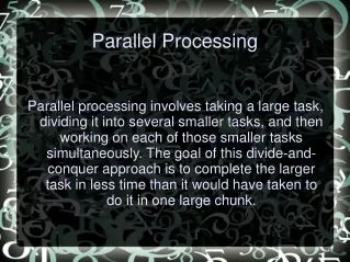
This comprehensive guide delves into the necessity of multi-core/processor parallel processing in the context of Moore's Law limitations. It explores various uni-processor performance enhancement techniques, applications, computation classifications, parallel architectures, and MIMD/SPMD algorithms. Additionally, it reviews the fundamentals of parallel processing, pipelining, cache systems, and the quest for high performance. The text emphasizes the need for explicit parallel algorithms to optimize performance effectively.

E N D
Introduction to Parallel Processing Shantanu Dutt University of Illinois at Chicago
Acknowledgements • Ashish Agrawal, IIT Kanpur, “Fundamentals of Parallel Processing” (slides), w/ some modifications and augmentations by Shantanu Dutt • John Urbanic, Parallel Computing: Overview (slides), w/ some modifications and augmentations by Shantanu Dutt • John Mellor-Crummey, “COMP 422 Parallel Computing: An Introduction”, Department of Computer Science, Rice University, (slides), w/ some modifications and augmentations by Shantanu Dutt
Outline • The need for explicit multi-core/processor parallel processing: • Moore's Law and its limits • Different uni-processor performance enhancement techniques and their limits • Applications for parallel processing • Overview of different applications • Classification of parallel computations • Classification of parallel architectures • Examples of MIMD/SPMD parallel algorithms • Summary Some text from: Fund. of Parallel Processing, A. Agrawal, IIT Kanpur
Outline • The need for explicit multi-core/processor parallel processing: • Moore's Law and its limits • Different uni-processor performance enhancement techniques and their limits • Applications for parallel processing • Overview of different applications • Classification of parallel computations • Classification of parallel architectures • Examples of MIMD/SPMD parallel algorithms • Summary Some text from: Fund. of Parallel Processing, A. Agrawal, IIT Kanpur
Moore’s Law & Need for Parallel Processing • Chip performance doubles every 18-24 months • Power consumption is prop. to freq. • Limits of Serial computing – • Heating issues • Limit to transmissions speeds • Leakage currents • Limit to miniaturization • Multi-core processors already commonplace. • Most high performance servers already parallel. Fundamentals of Parallel Processing, Ashish Agrawal, IIT Kanpur
Fundamentals of Parallel Processing, Ashish Agrawal, IIT Kanpur Quest for Performance • Pipelining • Superscalar Architecture • Out of Order Execution • Caches • Instruction Set Design Advancements • Parallelism • Multi-core processors • Clusters • Grid This is the future
Pipelining • Illustration of Pipeline using the fetch, load, execute, store stages. • At the start of execution – Wind up. • At the end of execution – Wind down. • Pipeline stalls due to data dependency (RAW, WAR), resource conflict, incorrect branch prediction – Hit performance and speedup. • Pipeline depth – No of cycles in execution simultaneously. • Intel Pentium 4 – 35 stages. Top text from: Fundamentals of Parallel Processing, A. Agrawal, IIT Kanpur
Pipelining • Tpipe(n) is pipelined time to process n instructions = fill-time + n*(max{ti} ~ n*(max{ti} for large n, as fill-time is a constant wrt n), ti = exec. time of the i’th stage. • This pipelined throughput = 1/max{ti}
Cache • Desire for fast cheap and non volatile memory • Memory speed growth at 7% per annum while processor growth at 50% p.a. • Cache – fast small memory. • L1 and L2 caches. • Retrieval from memory takes several hundred clock cycles • Retrieval from L1 cache takes the order of one clock cycle and from L2 cache takes the order of 10 clock cycles. • Cache ‘hit’ and ‘miss’. • Prefetch used to avoid cache misses at the start of the execution of the program. • Cache lines used to avoid latency time in case of a cache miss • Order of search – L1 cache -> L2 cache -> RAM -> Disk • Cache coherency – Correctness of data. Important for distributed parallel computing • Limit to cache improvement: Improving cache performance will at most improve efficiency to match processor efficiency Fundamentals of Parallel Processing, Ashish Agrawal, IIT Kanpur
: instruction-level parallelism—degree generally low and dependent on how the sequential code has been written, so not v. effective (single-instr. multiple data) (exs. of limited data parallelism) (exs. of limited & low-level functional parallelism)
(simultaneous multi- threading) (multi-threading)
Thus ……: Two Fundamental Issues in Future High Performance Fundamentals of Parallel Processing, Ashish Agrawal, IIT Kanpur Microprocessor performance improvement via various implicit and explicit parallelism schemes and technology improvements is reaching (has reached?) a point of diminishing returns Thus need development of explicit parallel algorithms that are based on a fundamental understanding of the parallelism inherent in a problem, and exploiting that parallelism with minimum interaction/communication between the parallel parts
Outline • The need for explicit multi-core/processor parallel processing: • Moore's Law and its limits • Different uni-processor performance enhancement techniques and their limits • Applications for parallel processing • Overview of different applications • Classification of parallel computations • Classification of parallel architectures • Examples of MIMD/SPMD parallel algorithms • Summary Some text from: Fund. of Parallel Processing, A. Agrawal, IIT Kanpur
Computing and Design/CAD Designs of complex to very complex systems have almost become the norm in many areas of engineering, from design of chips with billions of transistors to aircrafts of various types of sophistication (large fly-by-wire passenger aircrafts to fighter planes) to complex engines to buildings and bridges. An effective design process needs to explore the design space in smart ways (without being exhaustive but also without leaving out useful design points) to optimize some metric (e.g., minimizing power consumption of a chip) while satisfying tens to hundreds of constraints on others (e.g., on speed and temperature profile of the chip). This is an extremely time intensive process for large and complex designs and can benefit significantly from parallel processing.
Applications of Parallel Processing Fundamentals of Parallel Processing, Ashish Agrawal, IIT Kanpur
Fundamentals of Parallel Processing, Ashish Agrawal, IIT Kanpur
Outline • The need for explicit multi-core/processor parallel processing: • Moore's Law and its limits • Different uni-processor performance enhancement techniques and their limits • Applications for parallel processing • Overview of different applications • Classification of parallel computations • Classification of parallel architectures • Examples of MIMD/SPMD parallel algorithms • Summary and future advances Some text from: Fund. of Parallel Processing, A. Agrawal, IIT Kanpur
Parallelism - A simplistic understanding • Multiple tasks at once. • Distribute work into multiple execution units. • A classification of parallelism: • Data Parallelism • Functional or Control Parallelism • Data Parallelism - Divide the dataset and solve each sector “similarly” on a separate execution unit. • Functional Parallelism – Divide the 'problem' into different tasks and execute the tasks on different units. What would func. parallelism look like for the example on the right? • Hybrid: Can do both: Say, first partition by data, and then for each data block, partition by functionality Sequential Data Parallelism Fundamentals of Parallel Processing, Ashish Agrawal, IIT Kanpur
Data Parallelism Functional Parallelism: Example: Earth weather model Q: What would a data parallel breakup look like for this problem? Q. How can a hybrid breakup be done? • The “trick” for either type of parallelism is partitioning the problem (by data, tasks/functions, or both) so that: (a) There is minimum communication between partitions (i.e., between processors working on these partitions); communication is an overhead of parallel processing. (b) The amount of work in each partition is close to uniform so that no processor idles much until the computation is completed; idling is an overhead of parallel processing. (from S. Dutt) Fundamentals of Parallel Processing, Ashish Agrawal, IIT Kanpur
Flynn’s Classification • Flynn's Classical Taxonomy – Based on # of instruction/task and data streams • Single Instruction, Single Data streams (SISD): your single-core uni-processor PC • Single Instruction, Multiple Data streams (SIMD): special purpose low-granularity multi-processor m/c w/ a single control unit relaying the same instruction to all processors (w/ different data) every cc (e.g., nVIDIA graphic co-processor w/ 1000’s of simple cores) • Multiple Instruction, Single Data streams (MISD): pipelining is a major example • Multiple Instruction, Multiple Data streams (MIMD): the most prevalent model. SPMD (Single Program Multiple Data) is a very useful subset. Note that this is v. different from SIMD. Why? • Data vs Control Parallelism is an independent classification to Flynn’s Fundamentals of Parallel Processing, Ashish Agrawal, IIT Kanpur
Flynn’s Classification (cont’d). Example machines: Thinking Machines CM 2000, nVIDIA GPU
Flynn’s Classification (cont’d). Example machines: Various current multicomputers (see the most recent list at http://www.top500.org/), multi-core processors like the Intel i3, i5, i7 processors (all quad-core: 4 processors on a single chip)
Flynn’s Classification (cont’d). • Data Parallelism: SIMD and SPMD (seen at the high-level functional level, not at the atomic/low-level instruction level) fall into this category • Functional Parallelism: MISD falls into this category • MIMD can incorporate both data and functional parallelisms (the latter at either instruction level—different instrs. being executed across the processors at any time, or at the high-level function space)
Outline • The need for explicit multi-core/processor parallel processing: • Moore's Law and its limits • Different uni-processor performance enhancement techniques and their limits • Applications for parallel processing • Overview of different applications • Classification of parallel computations • Classification of parallel architectures • Examples of MIMD/SPMD parallel algorithms • Summary Some text from: Fund. of Parallel Processing, A. Agrawal, IIT Kanpur
Fundamentals of Parallel Processing, Ashish Agrawal, IIT Kanpur Multi-processor Architectures- Distributed Memory with message passing—Most prevalent architecture model for # processors > 8 Indirect interconnectionn n/ws Direct interconnection n/ws Shared Memory Uniform Memory Access (UMA) Non- Uniform Memory Access (NUMA)—Distributed shared memory 1 Parallel Arch. Classification
Distributed Memory—Message Passing Architectures • Each processor P (with its own local cache C) is connected to exclusive local memory, i.e. no other CPU has direct access to it. • Each node comprises at least one network interface (NI or routing switch) that mediates the connection to a communication network. • On each CPU runs a serial process that can communicate with other processes on other CPUs by means of the network. • Blocking vs Non-blocking communication • Blocking: computation stalls until commun. occurs/completes • Non-blocking: if no commun. has occurred/completed at calling point, computation proceeds to the next instruction/statement (may require later calls to commun. primitive, esp. for “receive”, until commun. occurrs) • Direct vs Indirect Communication / Interconnection network Example: A 2x4 mesh n/w (direct connection n/w) Fundamentals of Parallel Processing, Ashish Agrawal, IIT Kanpur
The Extreme HPC at UIC (see https://acer.uic.edu/services/tutorials/)
1 System Computational Actions in a Message-Passing Program Process P1 Process P2 Process P1 Process P2 Message passing mapping a := b+c; b := x*y; recv(P2, b); /* blocking */ a := b+c; b := x*y; send(P1,b); /* non-blocking */ (a) Two basic parallel processes P1, P2, and their data dependency b Processor/core containing P1 Processor/core containing P2 P(P1) P(P2) Message passing of data item “b”. Link(s) (direct or indirect) betw. the 2 processors (b) Their mapping to a message-passing multicomputer
1 Uniform Shared Memory Arch.: UMA • Flat memory model • Memory bandwidth and latency are the same for all processors and all memory locations. • Simplest example – dual core processor • Most commonly represented today by Symmetric Multiprocessor (SMP) machines • Cache coherent UMA—consistent cache values of the same data item in different proc./core caches L1 cache L2 cache Dual-Core Quad-Core Fundamentals of Parallel Processing, Ashish Agrawal, IIT Kanpur
1 System Computational Actions in a Shared-Memory Program Process P1 Process P1 Process P2 Process P2 Shared-memory mapping Possible Actions by O.S.: (i) Since “b” is a shared data item (e.g., designated by compiler or programmer), check “b”’s location to see if it can be written to (all reads done: read_cntr for “b” = 0). (ii) If so, write “b” to its location and mark status bit as written by “P2”. (or increment its write counter if “b” will be written to multiple times by “P2”). (iii) Initialize read_cntr for “b” to pre-determined value (# of procs. to read it) Possible Actions by O.S.: (i) Since “b” is a shared data item (e.g., designated by compiler or programmer), check “b”’s status bit to see if it has been written to (or more generally, check if a write counter is incremented since last read—locally store write counter value for each read) (ii) If so {read “b” & decrement read_cntr for “b”} else go to (i) and busy wait (check periodically) if blocking, else do some other work and check back later. a := b+c; b := x*y; b := x*y; a := b+c; (a) Two basic parallel processes P1, P2, and their data dependency P(P1) P(P2) Shared Memory (b) Their mapping to a shared-memory multiprocessor