Download
1 / 35
350 likes | 357 Views
Recap from Monday. Frequency domain analytical tool computational shortcut compression tool. Fourier Transform in 2d. in Matlab, check out: imagesc(log(abs(fftshift(fft2(im)))));. Image Blending (Szeliski 9.3.4). Google Street View. CS129: Computational Photography

E N D
Recap from Monday Frequency domain analytical tool computational shortcut compression tool
Fourier Transform in 2d in Matlab, check out: imagesc(log(abs(fftshift(fft2(im)))));
Image Blending (Szeliski 9.3.4) Google Street View CS129: Computational Photography James Hays, Brown, Spring 2011 Many slides from Alexei Efros
Compositing Procedure 1. Extract Sprites (e.g using Intelligent Scissors in Photoshop) 2. Blend them into the composite (in the right order) Composite by David Dewey
+ = 1 0 1 0 Alpha Blending / Feathering Iblend = aIleft + (1-a)Iright
Setting alpha: simple averaging Alpha = .5 in overlap region
Setting alpha: center seam Distance Transform bwdist Alpha = logical(dtrans1>dtrans2)
Setting alpha: blurred seam Distance transform Alpha = blurred
Ghost! Setting alpha: center weighting Distance transform Alpha = dtrans1 / (dtrans1+dtrans2)
0 1 0 1 Affect of Window Size left right
0 1 0 1 Affect of Window Size
0 1 Good Window Size “Optimal” Window: smooth but not ghosted
Band-pass filtering • Laplacian Pyramid (subband images) • Created from Gaussian pyramid by subtraction Gaussian Pyramid (low-pass images)
Laplacian Pyramid • How can we reconstruct (collapse) this pyramid into the original image? Need this! Original image
0 1 0 1 0 1 Pyramid Blending Left pyramid blend Right pyramid
laplacian level 4 laplacian level 2 laplacian level 0 left pyramid right pyramid blended pyramid
Laplacian Pyramid: Blending • General Approach: • Build Laplacian pyramids LA and LB from images A and B • Build a Gaussian pyramid GR from selected region R • Form a combined pyramid LS from LA and LB using nodes of GR as weights: • LS(i,j) = GR(I,j,)*LA(I,j) + (1-GR(I,j))*LB(I,j) • Collapse the LS pyramid to get the final blended image
Horror Photo david dmartin (Boston College)
Simplification: Two-band Blending • Brown & Lowe, 2003 • Only use two bands: high freq. and low freq. • Blends low freq. smoothly • Blend high freq. with no smoothing: use binary alpha
Don’t blend, CUT! (project 4) • So far we only tried to blend between two images. What about finding an optimal seam?
2 _ = overlap error min. error boundary Project 3 and 4 -Minimal error boundary overlapping blocks vertical boundary
Graphcuts • What if we want similar “cut-where-things-agree” idea, but for closed regions? • Dynamic programming can’t handle loops
a cut hard constraint n-links hard constraint t s Graph cuts (simple example à la Boykov&Jolly, ICCV’01) Minimum cost cut can be computed in polynomial time (max-flow/min-cut algorithms)
Kwatra et al, 2003 Actually, for this example, dynamic programming will work just as well…
Gradient Domain Image Blending • In Pyramid Blending, we decomposed our image into 2nd derivatives (Laplacian) and a low-res image • Let’s look at a more direct formulation: • No need for low-res image • captures everything (up to a constant) • Idea: • Differentiate • Composite • Reintegrate
Gradient Domain blending (1D) bright Two signals dark Regular blending Blending derivatives
Gradient Domain Blending (2D) • Trickier in 2D: • Take partial derivatives dx and dy (the gradient field) • Fidle around with them (smooth, blend, feather, etc) • Reintegrate • But now integral(dx) might not equal integral(dy) • Find the most agreeable solution • Equivalent to solving Poisson equation • Can use FFT, deconvolution, multigrid solvers, etc.
Perez et al, 2003 • Limitations: • Can’t do contrast reversal (gray on black -> gray on white) • Colored backgrounds “bleed through” • Images need to be very well aligned editing
Putting it all together • Compositing images • Have a clever blending function • Feathering • Center-weighted • blend different frequencies differently • Gradient based blending • Choose the right pixels from each image • Dynamic programming – optimal seams • Graph-cuts • Now, let’s put it all together: • Interactive Digital Photomontage, 2004 (video)