Download
1 / 26
270 likes | 565 Views
CS 4731: Computer Graphics Lecture 23: Curves. Emmanuel Agu. So Far…. Dealt with straight lines and flat surfaces Real world objects include curves Need to develop: Representations of curves Tools to render curves. Curve Representation: Explicit. One variable expressed in terms of another

E N D
CS 4731: Computer GraphicsLecture 23: Curves Emmanuel Agu
So Far… • Dealt with straight lines and flat surfaces • Real world objects include curves • Need to develop: • Representations of curves • Tools to render curves
Curve Representation: Explicit • One variable expressed in terms of another • Example: • Works if one x-value for each y value • Example: does not work for a sphere • Rarely used in CG because of this limitation
Curve Representation: Implicit • Algebraic: represent 2D curve or 3D surface as zeros of a formula • Example: sphere representation • May restrict classes of functions used • Polynomial: function which can be expressed as linear combination of integer powers of x, y, z • Degree of algebraic function: highest sum of powers in function • Example: yx4 has degree of 5
Curve Representation: Parametric • Represent 2D curve as 2 functions, 1 parameter • 3D surface as 3 functions, 2 parameters • Example: parametric sphere
Choosing Representations • Different representation suitable for different applications • Implicit representations good for: • Computing ray intersection with surface • Determing if point is inside/outside a surface • Parametric representation good for: • Breaking surface into small polygonal elements for rendering • Subdivide into smaller patches • Sometimes possible to convert one representation into another
Continuity • Consider parametric curve • We would like smoothest curves possible • Mathematically express smoothness as continuity (no jumps) • Defn: if kth derivatives exist, and are continuous, curve has kth order parametric continuity denoted Ck
Continuity • 0th order means curve is continuous • 1st order means curve tangent vectors vary continuously, etc • We generally want highest continuity possible • However, higher continuity = higher computational cost • C2 is usually acceptable
Interactive Curve Design • Mathematical formula unsuitable for designers • Prefer to interactively give sequence of control points • Write procedure: • Input: sequence of points • Output: parametric representation of curve
Interactive Curve Design • 1 approach: curves pass through control points (interpolate) • Example: Lagrangian Interpolating Polynomial • Difficulty with this approach: • Polynomials always have “wiggles” • For straight lines wiggling is a problem • Our approach: merely approximate control points (Bezier, B-Splines)
De Casteljau Algorithm • Consider smooth curve that approximates sequence of control points [p0,p1,….] • Blending functions: u and (1 – u) are non-negative and sum to one
De Casteljau Algorithm • Now consider 3 points • 2 line segments, P0 to P1 and P1 to P2
De Casteljau Algorithm Example: Bezier curves with 3, 4 control points
De Casteljau Algorithm Blending functions for degree 2 Bezier curve Note: blending functions, non-negative, sum to 1
De Casteljau Algorithm • Extend to 4 points P0, P1, P2, P3 • Repeated interpolation is De Casteljau algorithm • Final result above is Bezier curve of degree 3
De Casteljau Algorithm • Blending functions for 4 points • These polynomial functions called Bernstein’s polynomials
De Casteljau Algorithm • Writing coefficient of blending functions gives Pascal’s triangle 1 1 1 1 2 1 1 1 3 3 1 4 6 4 1 In general, blending function for k Bezier curve has form where
De Casteljau Algorithm • Can express cubic parametric curve in matrix form where
Subdividing Bezier Curves • OpenGL renders flat objects • To render curves, approximate by small linear segments • Subdivide curved surface to polygonal patches • Bezier curves useful for elegant, recursive subdivision • May have different levels of recursion for different parts of curve or surface • Example: may subdivide visible surfaces more than hidden surfaces
Subdividing Bezier Curves • Let (P0… P3) denote original sequence of control points • Relabel these points as (P00…. P30) • Repeat interpolation (u = ½) and label vertices as below • Sequences (P00,P01,P02,P03) and (P03,P12,P21,30) define Bezier curves also • Bezier Curves can either be straightened or curved recursively in this way
Bezier Surfaces • Bezier surfaces: interpolate in two dimensions • This called Bilinear interpolation • Example: 4 control points, P00, P01, P10, P11, 2 parameters u and v • Interpolate between • P00 and P01 using u • P10 and P11 using u • Repeat two steps above using v
Bezier Surfaces • Recalling, (1-u) and u are first-degree Bezier blending functions b0,1(u) and b1,1(u) Generalizing for cubic Rendering Bezier patches in openGL: v=u = 1/2
B-Splines • Bezier curves are elegant but too many control points • Smoother = more control points = higher order polynomial • Undesirable: every control point contributes to all parts of curve • B-splines designed to address Bezier shortcomings • Smooth blending functions, each non-zero over small range • Use different polynomial in each range, (piecewise polynomial) B-spline blending functions, order 2
NURBS • Encompasses both Bezier curves/surfaces and B-splines • Non-uniform Rational B-splines (NURBS) • Rational function is ratio of two polynomials • NURBS use rational blending functions • Some curves can be expressed as rational functions but not as simple polynomials • No known exact polynomial for circle • Rational parametrization of unit circle on xy-plane:
NURBS • We can apply homogeneous coordinates to bring in w • Using w, we get we cleanly integrate rational parametrization • Useful property of NURBS: preserved under transformation • Thus, we can project control points and then render NURBS
References • Hill, chapter 11