Download
1 / 53
550 likes | 791 Views
Integrating GIS and environmental models. integrated tools for spatial environmental analysis. Integrating GIS. GIS are computer based tools to: capture, manipulate, process, and display spatial or geo-referenced data. Integrating GIS. They combine

E N D
Integrating GIS and environmental models integrated tools for spatial environmental analysis K.Fedra ‘97
Integrating GIS ... GIS are computer based tools to: • capture, • manipulate, • process, and • display spatial or geo-referenced data. K.Fedra ‘97
Integrating GIS ... They combine • geometry data (coordinates and topological information) and • attribute data, describing the properties of geometrical objects (points, lines, areas) • with tools for spatial (geometric) analysis. K.Fedra ‘97
Integrating GIS ... Environmental problems are spatial problems, environmental data can almost always be georeferenced. GIS is therefor an appropriate tool for environmental analysis. K.Fedra ‘97
Integrating GIS ... Basic concepts in GIS are: • location • spatial distribution • spatial relationship Basic elements: • spatial objects K.Fedra ‘97
Integrating GIS ... Basic concepts in environmental modeling are: • systems state • systems dynamics • interaction Basic elements: • functional objects and processes K.Fedra ‘97
Merging Paradigms Overlap and relationship between GIS and environmental models is apparent, so the merging of the two fields of research, technologies, or sets of methods, their paradigms, is an obvious and promising idea. K.Fedra ‘97
Merging Paradigms Datafile GIS ENV GIS+ENV SocSciSearch 181 9,898 6 SciSearch 143 6,118 7 Enviroline 121 25,310 34 WaterRes. 165 44,696 56 Computer DB 501 21,933 81 266 INSPEC 1,711 105,781 Literature search from summer 1991 K.Fedra ‘97
Environmental Modeling: a mathematical representation of environmental processes, and relationships. Digital (numerical) Analog computers Scale models K.Fedra ‘97
Environmental Modeling considerable tradition: • 1856 Darcy’s Law, fundamental equation describing groundwater flow • 1871 St.Venant equations describing unsteady open channel flow • 1924 Lotka’s Elements of Physical Biology K.Fedra ‘97
Environmental Modeling • 1960-70 first computer models • 1971 B.Patten, Systems Analysis and Simulation in Ecology (linear systems) • 1972 J.Forrester, Principles of Systems (Systems Dynamics) • 1972 H.T.Odum, Energy flow modeling • 1974,79 CLEANER multi-compartment lake models, Park et.al. K.Fedra ‘97
Environmental Modeling Development through increasing complexity: number of interacting compartments, types of interactions. No explicit spatial distribution in early process models. First spatially explicit models in the physical domain (flow), linkage of transport and ecological processes by the mid 70’s and 80’s. K.Fedra ‘97
Environmental Modeling Simplified block diagram of the aquatic ecosystem model CLEANER (Park et al., 1975) K.Fedra ‘97
Types of Models • scale models (architecture, construction, mechanical engineering) • conceptual models (qualitative, block and flow diagrams, show major components and interrelationships) • mathematical models: • analytical, analog, digital K.Fedra ‘97
Types of Models • scale models (architecture, construction, mechanical engineering) • conceptual models (qualitative, block and flow diagrams, show major components and interrelationships) • mathematical models K.Fedra ‘97
Types of Models mathematical models • conceptual or empirical • deterministic or stochastic • steady-state or dynamic • analytical or numerical • spatially aggregated or distributed K.Fedra ‘97
Types of Models • conceptual or empirical • based on basic laws of nature or theoretical concepts • derived from observations (input-output relations), providing phenomenological descriptions K.Fedra ‘97
Types of Models • deterministic or stochastic • all model inputs and parameters are assumed to be exactly known • inputs and parameters can be represented by probability distributions, resulting in probabilistic state and output K.Fedra ‘97
Types of Models • steady-state or dynamic • input and parametes are time-invariant, a solution independent of time can be derived • some model elements are described as functions of time K.Fedra ‘97
Types of Models • analytical or numerical • the model equations can be solved analytically and exactly • equations require a numerical approximation for solution, based on some form of discretization K.Fedra ‘97
Types of Models • spatially aggregated or distributed • model is assumed to be independent of spatial location • models uses average (lumped) values to describe a larger area • inputs, parameters or the transfer function vary with location, state is defined for more than one location, spatial elements interact K.Fedra ‘97
Modeling Domains • Atmospheric systems • Hydrologic systems • Land surface and subsurface • Biological and ecological systems • Risks and hazards • Management and policy models K.Fedra ‘97
Modeling Domains • Atmospheric systems • weather forecasting • climate models • air pollution: industry, traffic, domestic sources, accidental releases (hazardous substances) K.Fedra ‘97
Modeling Domains • Air pollution modeling • estimation of the source term: • rate and duration of release • source size, location • initial buoyancy and momentum K.Fedra ‘97
Modeling Domains • Air pollution modeling • pollutant transport • advection by wind • turbulent and molecular diffusion • buoyancy effects (gases, particles) • deposition, chemical reactions, radioactive decay K.Fedra ‘97
Modeling Domains • Air pollution modeling • impacts and hazards • human end environmental exposure • damage through explosion and fire • damage through chemical reactions (corrosion) K.Fedra ‘97
Modeling Domains • Hydrologic systems • hydrological cycle, rainfall-runoff • river flow and flooding • water distribution and allocation • reservoir operations • water quality, eutrophication, waste allocation • groundwater systems K.Fedra ‘97
Modeling Domains • Coastal waters and oceans • currents and energy balance (climate modeling) • coastal water quality • nutrient cycles, eutrophication • fisheries (sustainable yield) K.Fedra ‘97
Modeling Domains • Land surface and subsurface • erosion, soil processes • vegetation, land cover • groundwater (unsaturated and saturated zones, links to the hydrological domain) K.Fedra ‘97
Modeling Domains • Biological and ecological systems • population models, predator-prey systems, food chains • ecosystem models (multi-compartment combining physical and biological elements) K.Fedra ‘97
Modeling Domains • Agriculture and Forestry • agricultural production • livestock and grazing models • forest models (stands, growth, yield, deforestation and reforestation) K.Fedra ‘97
Modeling Domains • Risks and hazards • floods and droughts • erosion, desertification • spills and accidental releases • epidemiological models (pests, infectuous diseases) K.Fedra ‘97
Modeling Domains • Management and policy models • all of the above, but containing explicit representation of control and decision variables • economic evaluation K.Fedra ‘97
Modeling Domains All environmental model domains have an obvious spatial dimension. Most recent environmental models are spatially explicit (inputs and state are functions of space) X (x,y,z,t) K.Fedra ‘97
Distributed Models are based on partial differential equations; dependent variables are functions of two or more other variables: dQ dQ dx dy (continuity equation for 2D groundwater flow) = 0 + K.Fedra ‘97
Distributed Models and the partial differentials dQ/dx and dQ/dy describe the gradient of discharge Qin the horizontal x and y directions. K.Fedra ‘97
Distributed Models The partial differential equations are solved with a numerical scheme like finite elements or finite differences. This requires the solution domain to be discretized. K.Fedra ‘97
Distributed Models Process equations are solved for each of the discrete units in the model domain. K.Fedra ‘97
Distributed Models coupling of cells is achieved through transfer processes such as advection and diffusion. K.Fedra ‘97
Merging Paradigms Use GIS functionality for data capture, processing and display; Use GIS functionality for static, geometric analysis; Use model functionality for dynamic processes and complex analysis. K.Fedra ‘97
GIS-Model coupling • data exchange between two separate systems • common interface, shared data • common interface, fully integrated functionality K.Fedra ‘97
GIS-Model coupling • data exchange between two separate systems: • GIS acts as a pre- and post-processor for a dynamic environmental model. K.Fedra ‘97
GIS-Model coupling shared files GIS MODEL user interface user interface separate user interfaces, shared files K.Fedra ‘97
GIS-Model coupling shared files and memory GIS MODEL common user interface common user interface, shared files and memory K.Fedra ‘97
GIS-Model coupling full integration of GIS and models together with a DSS component representing a problem-oriented user interface. GIS MODELS DSS K.Fedra ‘97
GIS-Model coupling data files rule base GIS DBMS KB pre- processor post- processor MODELS help/explain visualization scenario manager interactive user interface K.Fedra ‘97
Example: groundwater modeling Spatially distributed aquifer characteristics (conductivity, porosity) and inputs (recharge) are derived from appropriate maps; Model output is displayed as (animated) map overlays. K.Fedra ‘97
K.Fedra ‘97 from a digitized geological map …...
K.Fedra ‘97 a rasterized data set of aquifer properties is derived ...
K.Fedra ‘97 The map is background and input to the model ...