Download
1 / 38
470 likes | 700 Views
R- Tree. Spatial Database ( Ia ). Consider: Given a city map, ‘index’ all university buildings in an efficient structure for quick topological search. Spatial Database (Ib). Consider: Given a city map, ‘index’ all university buildings in an efficient structure for quick topological search.

E N D
Spatial Database (Ia) • Consider: Given a city map, ‘index’ all university buildings in an efficient structure for quick topological search.
Spatial Database (Ib) • Consider: Given a city map, ‘index’ all university buildings in an efficient structure for quick topological search. Spatial object: Contour (outline) of the area around the building(s). Minimum bounding region (MBR) of the object.
Spatial Database (Ic) • Consider: Given a city map, ‘index’ all university buildings in an efficient structure for quick relational-topological search. MBR of the city neighbourhoods. MBR of the city defining the overall search region.
Spatial Database (II) Notion: To retrieve data items quickly and efficiently according to their spatial locations. • Involves 2D regions. • Need to support 2D range queries. • Multiple return values desired: Answering a query region by reporting all spatial objects that are fully-contained-in or overlapping the query region (Spatial-Access Method – SAM). In general: • Spatial data objects often cover areas in multidimensional spaces. • Spatial data objects are not well-represented by point-location. • An ‘index’ based on an object’s spatial location is desirable.
M E H P T X B D F G I K L N O Q S V W Y Z The Indexing Approach • A B-Tree (Rosenberg & Snyder, 1981) is an ordered, dynamic, multi-way structure of order m (i.e. each node has at most m children). • The keys and the subtrees are arranged in the fashion of a search tree. • Each node may contain a large number of keys, and the number of subtrees in each node, then, may also be large. • The B-Tree is designed (among other objectives): • to branch out this large number of directions, and • to contain a lot of keys in each node so that the height of the tree is relatively short.
The R-Tree Index Structure • An R-Tree is a height-balanced tree, similar to a B-Tree. • Index records in the leaf nodes contain pointers to the actual spatial-objects they represent. • Leaves in the structure all appear on the same level. • Spatial searching requires visiting only a small number of nodes. • The index is completely dynamic: inserts and deletes can be intermixed with searches. • No periodic reorganisation is required.
The R-Tree Index Structure • A spatial database consists of a collection of tuples representing spatial objects, known as Entries. • Each Entry has a unique identifier that points to one spatial object, and its MBR; i.e. Entry = (MBR, pointer).
R-Tree Index Structure – Leaf Entries • An entryE in a leaf node is defined as (Guttman, 1984): E = (I, tuple-identifier) • Where I refers to the smallest bindingn-dimensional region (MBR) that encompasses the spatial data pointed to by its tuple-identifier. • I is a series of closed-intervals that make up each dimension of the binding region. Example. In 2D, I = (Ix, Iy), where Ix = [xa, xb], and Iy = [ya, yb].
R-Tree Index Structure – Leaf Entries • In general I = (I0, I1, …, In-1) for n-dimensions, and that Ik = [ka, kb]. • If either ka or kb (or both) are equal to , this means that the spatial object extends outward indefinitely along that dimension.
B c I(A) I(a) I(B) I(b) … I(c) I(M) I(d) d b a R-Tree Index Structure – Non-Leaf Entries • An entryE in a non-leaf node is defined as: E = (I, child-pointer) • Where the child-pointer points to the child of this node, and I is the MBR that encompasses all the regions in the child-node’s pointer’s entries.
Properties Let M be the maximum number of entries that will fit in one node. Let m≤ M/2 be a parameter specifying the minimum number of entries in one node. Then an R-Tree must satisfy the following properties: • Every leaf node contains between m and M index records, unless it is the root. • For each index-record Entry (I, tuple-identifier) in a leaf node, I is the MBR that spatially contains the n-dimensional data object represented by the tuple-identifier. • Every non-leaf node has between m and M children, unless it is the root. • For each Entry (I, child-pointer) in a non-leaf node, I is the MBR that spatially contains the regions in the child node. • The root has two children unless it is a leaf. • All leaves appear on the same level.
Node Overflow and Underflow • A Node-Overflow happens when a new Entry is added to a fully packed node, causing the resulting number of entries in the node to exceed the upper-boundM. • The ‘overflow’ node must be split, and all its current entries, as well as the new one, consolidated for local optimum arrangement. • A Node-Underflow happens when one or more Entries are removed from a node, causing the remaining number of entries in that node to fall below the lower-boundm. • The underflow node must be condensed, and its entries dispersed for global optimum arrangement.
Spatial Indexes Used to speed up spatial queries Example: Point query: return the geometric object that contains a given query point Sequentially scanning all objects of a large collection to check whether they contain the query point involves a high number of disk accesses and the repetition of the evaluation of computationally expensive geometric predicates (e.g., containment, intersection, etc.) Reducing the set of objects to be processed is highly desirable
Indexes for object-based and space-based representations Indexes for raster data: based on recursive subdivision of the space Example: quadtrees Indexes for vector data: differ depending on the type of data (extensions of quadtrees are used also for vector data)
Vector Data Indexing • Different indexing methods are used for point, linear and polygonal data • In the case of collections of polygons, instead of indexing the object geometries themselves, whose shapes might be complex, we consider an approximation of the geometry and index it instead • Most commonly used approximation: minimum bounding rectangle (MBR) also called minimum bounding box (MBB)
MBRs • By using the MBR as the geometric key for building the spatial index, we save the cost of evaluating expensive geometric predicates during index traversal (as geometric tests againsts an MBR is constant) • Example: point-in-polygon test • In addition, the space required to store a rectangle is constant (2 points) (x,y) (x,y)
MBRs (cont.d) • An operation involving a spatial predicate on a collection of objects indexed on their MBRs is performed in two steps: • Filter step: selects the objects whose MBR satisfies the spatial predicate (by traversing the spatial index and applying the predicate to the MBRs) • Refinement step: the objects that pass the filter step are a superset of the solution. An MBR might satisfy the predicate but the corresponding object might not P MBR obj
Refinement step Refinement step: the objects that pass the filter step are a superset of the solution. An MBR might satisfy the predicate but the corresponding object might not Therefore, in this step the spatial predicate is applied to the actual geometry of the object P MBR obj
Spatial LayerData Secondary Filter Spatial Functions Primary Filter Spatial Index Reduced Data Set Table where coordinates are stored Index retrieves area of interest Procedures that determine exact relationship Oracle Spatial Query Model Exact Result Set
Oracle Spatial Indexing Methods Two types of indexes are implemented in Oracle Spatial: • R-trees • Quadtrees
R-trees Based on MBRs (minimum bounding rectangles) Defined for indexing 2D objects (can be extended to higher dimensions but implemented only for 2D in Oracle Spatial) MBRs of geometric objects form the leaves of the index tree Multiple MBRs are grouped into larger rectangles (MBRs) to form intermediate nodes in the tree Repeat until one rectangle is left that contains everything
a root R b R S d a b c d S c root 1 2 3 4 5 6 7 8 9 Pointers to geometries R-trees R-tree 1 2 3 4 8 6 5 9 7
Remark: nodes • Intermediate nodes store: • MBRs of collections of objects • Leaf nodes store: • MBRs of individual objects • Pointers to storage location of the exact geometry
Building R-trees An R-tree is a depth-balanced tree in which each node corresponds to a disk page (i.e., the number of entries in each node is limited) The structure satisfies the following properties: • For all nodes in the tree (except the root) the number of entries is between m and M • The root has at least two children (unless it is a leaf) • All leaves are at the same level
a root R b R S d a b c d S c root 1 2 3 4 5 6 7 8 9 Pointers to geometries Example (1) R-tree 1 2 3 4 8 6 5 9 7 m = 2; M = 3
root R2 R3 R1 ….. ….. ….. Example (2) R-tree m = 2; M = 4
Searching R-trees • We consider two types of queries: • point query: “what object contains the query point” • window query: “what objects intersect the query window”
O Basic spatial queries (1) P Containment Query: Given a spatial object O, find all objects in the collection that completely contain O. When O is a point, the query is called Point Query Containment Query Point Query (also Point-in-polygon, or Point Location)
Basic spatial queries (2) Region Query: Given a region R, find all objects in the collection that intersect R. When R is a rectangle, the query is called Window Query R R Region Query Window Query
Searching R-trees: window query • Compare search window with MBRs stored at each node • starting at root node • Stop at leaf nodes • compare contained geometries with search window
a root R b R S d a b c d S c root 1 2 3 4 8 9 Pointers to geometries Searching R-trees: window query Example: R-tree 1 2 3 4 8 6 5 9 7
Example: remarks If no MBRs are used: check the query window against all geometries for intersection (computationally expensive) In some cases, using R-trees to structure the set of MBRs can cause more tests (against MBRs) to be done. In general, this is not the case
Searching R-trees: point query Test query point for inclusion in MBRs stored at each node • starting at root node • Stop at leaf nodes • Test query point for inclusion in exact geometries
a root P R b R S d a b c d S c root 1 2 3 4 5 6 7 8 9 Pointers to geometries Exercise: point query R-tree 1 2 3 4 8 6 5 9 7
a root P R b R S a b S root 3 4 Pointers to geometries Searching R-trees: point query Example: R-tree 1 2 3 4 8 6 5 9 7
Summary • Indexing Vector Spatial Data • R-trees: • Based on MBRs (leaves) • Root: whole dataset • Intermediate nodes: groups of MBRs (objects) – not a partition of the underlying space!
Important remarks • Note that the MBRs (at all levels) can overlap • A rectangle is stored as child of a bigger rectangle only if completely contained in it • Example: