Download

1 / 29
290 likes | 422 Views
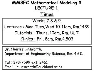
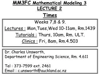
MM3FC Mathematical Modeling 3 LECTURE 10. Times Weeks 7,8 & 9. Lectures : Mon,Tues,Wed 10-11am, Rm.1439 Tutorials : Thurs, 10am, Rm. ULT. Clinics : Fri, 8am, Rm.4.503. Dr. Charles Unsworth, Department of Engineering Science, Rm. 4.611 Tel : 373-7599 ext. 8 2461

E N D
MM3FC Mathematical Modeling 3LECTURE 10 Times Weeks 7,8 & 9. Lectures : Mon,Tues,Wed 10-11am, Rm.1439 Tutorials : Thurs, 10am, Rm. ULT. Clinics : Fri, 8am, Rm.4.503 Dr. Charles Unsworth, Department of Engineering Science, Rm. 4.611 Tel : 373-7599 ext. 82461 Email : c.unsworth@auckland.ac.nz
This LectureWhat are we going to cover & Why ? • Spectral Analyser. • (Understand the DSP behind a spectrum analyser) • Discrete Fourier Transform (DFT). • (From understanding the spectrum analyser • we will learn a DFT can be represented as a filter bank) • Calculating a DFT. • Determine the ‘Magnitude spectrum’ of a complicated digitised sequence.
X0 X2* X2 X1* X1 X3* X3 w -w2 -w1 w1 w2 w3 -w3 0 - Spectral Analysis • The basic idea of spectral analysis is to create a system that will compute the values of the spectral components from the digital sequence of numbers x[n] • The general form for representing a real signal x[n] as a sum of complex exponentials is : • For the case where N=3, the spectrum would be : … (10.1)
However, an equivalent plot could be used to translate the –ve frequencies to their +ve alias frequencies, using : • e-jwn = ej2n e-jwn = ej(2 –jw)n • We will find this form of the spectrum useful when we discuss the DFT. X0 X2* X2 X1 X1* X3 X3* w w1 w2 w3 0 2 -w3 2 -w2 2 -w1 2
A Spectrum Analyser • The job of a “Spectrum Analyser” is to extract the frequency, magnitude and phase of each spectral component in x[n]. • The analyser will only have a finite number of electronic channels (N+1) to separate the spectral components into. • However, there is an infinite amount of frequencies that could exist in the range 0< w < 2 of the signal x[n]. • Thus, we must choose the frequencies of the spectral components that are going to be dedicated to each channel first. • So we will have to pick our frequencies ahead of time, independent of the signal. • Since there is a finite number of channels (N+1), one obvious is to cover the total 2 frequency range with equally spaced frequencies : wk = 2k/N • Thus, the spectrum is only an approximate representation. … (10.2)
Spectrum Analysis by Filtering • Each channel of the analyser must do two jobs : - Isolate the frequency of interest. - Compute the complex amplitude (Xk) for that frequency. • Isolating the frequency of interest Is suited to a BPF with a narrow passband. • Once x[n] is passed through the BPF we can measure the ouput for its amplitude and phase. • Rather than design individual BPF’s for each channel, we shall introduce the frequency-shifting property of the spectrum. (In this way, all channels can share the same filter).
Frequency-Shifting • The frequency of a complex exponential can be shifted if it is multiplied by another complex exponential. • Let the signal x[n] be multiplied by exp(-jwsn). • The entire spectrum of x[n] if shifted in the –ve direction by (ws). • The idea is to shift the desired frequency to the zero frequency position. … (10.3)
Thus, if we wanted to move the frequency (w1) to the zero frequency position. We would multiply x[n] by exp(-jw1n). • Thus, the power spectrum of x[n] below : • Would become the power spectrum of x[n] exp(-jw1n). X0 X2* X2 X1* X1 X3* X3 w -w2 -w1 w1 w2 w3 -w3 0 - X0 X2* X2 X1* X1 X3* X3 w -w3-w1 -w2-w1 w2-w1 w3-w1 -2w1 -w1 0
yw[n] x[n] xw[n] Linear Lowpass Filter e-jwn Channel Filters • Why have we translated the desired frequency to the w=0 position ? • Measurement at w=0 is equivalent to finding the average value of the signal with a lowpass filter. • When a lowpass filter extracts the DC component of the shifted spectrum it is actually measuring the complex amplitude of the shifted spectral components in x[n]. • A system for doing this must not only measure the average value but null out all other competing sinusoidal components. Preserves what’s at w=0 Places over spectrum SHIFTS spectrum By wto the left
Spectrum Analysis of Periodic Signals • A spectrum analyser will work perfectly for periodic signals. • The same approach can be used for non-periodic signals but will have approximation errors. • A periodic signal can be defined by the shifting property : x[n –N] = x[n] Where, N is the period. (i.e if we delay x[n] by N we will get x[n] again) • If a complex exponential is periodic with period N, • For the last equation to be true, • Equating exponents we get : wN = 2k, Thus any periodic exponential can be expressed as :
Once the period is specified we can create different complex exponential signals by changing the value of (k). However, there are actually only (N) different frequencies because : • So k has the range k = 0,1,2, …, N-1 • Spectrum of a Periodic Discrete-time Signal • If x[n] has period (N). Then its spectrum can contain only complex exponentials with the same period. Hence, the general representation of a periodic discrete-time signal x[n] is : • The range is from 0 to (N-1) as there are only N different frequencies. • The frequencies are all multiples of a common fundamental frequency • w = 2/N … (10.4)
Now we will change the notation in anticipation for the DFT. • We will replace Xk by X[ k]/N. Thus, • Later on, we will see that this is the inverse DFT. • Filtering with a running Sum • Earlier, we showed that FIR filters can calculate a ‘running sum’ or ‘running average’. • Let’s consider the L-point running sum with the difference equation : • As we can see all the co-efficients are equal to one. … (10.5)
Spectral component of interest Normalised frequency /2 -0.5 -0.2 -0.1 0.5 0.1 0 8 8 5 5 5 5 10 -0.5 -0.2 -0.1 0.5 0.1 0 -0.5 -0.1 0.5 -0.2 0.1 0 • Procedure is : Take a typical signal x[n] with power spectrum below • Shift desired spectral component to zero position. • Put through running sum filter. Gain = 10 Null Frequency response of a Running sum filter Null • Only the spectral component at zero position is preserved. 5x10 = 50 Spectral component of interest Is magnified by the gain of 10. All other components are nulled.
As we can see, the ‘running-sum’ FIR has nulls in its frequency response curve at w= 2k/L. • And this works very well for nulling out a signal if its constituient frequencies are also equally spaced. • If x[n] is periodic and • Running sum filter length = period of x[n] • y[n] is • A constant signal • Thus, for a periodic signal, each channel is composed of the filter combination below that produces one spectral component. • The structure is called a ‘filter bank’. yk[n] x[n] xk[n] N-point Running Sum Filter e-j(2k/N)n
The Discrete-Fourier Transform (D.F.T.) • The previous discussion is a roundabout way to describe the DFT. • The ‘Forward DFT’ (X[k])’ or ‘Analysis Equation’ is given below : • By substituting in x[n] we can calculate the spectral components X[k] can be found. • Similarly, the ‘Inverse DFT’ (x[n]) or ‘Synthesis Equation’ is given below : • By subsituting, in the spectral components X[k] we can synthesise the input signal x[n]. … (10.6) … (10.7)
y0[n] = X[0] x0[n] e-j(0)n y1[n] = X[1] x1[n] x[n] e-j(2/N)n yk[n] = X[k] xk[n] N-point Running Sum Filter N-point Running Sum Filter N-point Running Sum Filter N-point Running Sum Filter e-j(2k/N)n yN-1[n] = X[N-1] xN-1[n] e-j(2(N-1)/N)n • The filter bank of the DFT to compute X[k] for k=0,1,2,……,(N-1)
Thus, • We will use the DFT formulas for computation. • And the ‘filter-bank’ for interpretation and insight. • The DFT transforms an n-domain(or time-domain) signal • into its frequency-domain representation.
Computing the Forward DFT • So how do we go about computing the DFT and determining the Magnitude Spectrum from an input sequence x[n] ? • Consider a simple continuous sinusoid with a frequency f = 1Hz x(t) = cos(2(1)t) Thus, 1 period of the signal will occur in 1 second. And the one sided Magnitude spectrum will give a single peak at 1Hz. • Let’s see if the forward DFT can predict this ! Okay let’s sample the signal 8 times in 1 sec, fs= 8Hz and Ts=1/8 secs The digitised signal is therefore : x[n] = x(nTs) = cos(2nTs) = cos(2n(1/8)) = cos((/4)n) We have 8 samples, N=8 occurring when n = 0,1,2,3, …, (N-1 = 7)
1 /4 5/4 3/2 7/4 2 /2 3/4 Ts 1 450 1 • Using the forward DFT formula we will determine the spectral components.
For k=0, For k=1,
0 -1 1 0 • The best way to calculate what x[n] is multiplied is to identify the smallest increment that the exponential goes up in. Consider X[1] again : • The exponential power is always a multiple of /4. • In general the exponential power is a multiple of 2/no.samples • Next create a unit circle which is split up into these partitions. • Then at each of the multiples write in the values the exponent has at these positions. Values of x[n] at each position Unit circle in partitions
For k = 2, 0 -1 1 0 • We can read off the values from the unit circle to determine what the exponent value is.
For k=3, 0 -1 1 0
1 2 /4 5/4 3/2 7/4 /2 3/4 2 2 7/4 /4 5/4 3/2 /4 5/4 3/2 7/4 3/4 /2 /2 3/4 Ts Ts Ts 1 1 9/4 k=1 /4 increments k=2 /2 increments k=3 3/4 increments • So as (k) increases, the sample frequency decreases. • Also we are autocorrelating the sequence x[n] with differently sampled versions of itself.
We can write all of this in a matrix notation : Power of the exponent (e-j/4) n increases x[n] k increases Goes up in p/4 ’s Goes up in p/2 ’s Goes up in 3p/4 ’s Goes up in p ’s Goes up in 5p/4 ’s Goes up in 3p/2 ’s Goes up in 7p/4 ’s So only need to remember this bit really. • Now we can read off the unit circle the values at these frequencies.
0 -1 1 0 Reflection in the line of 1’s and –1’s
The One-sided Magnitude Spectrum of the Signal The actual frequency of the sequence |X| The ‘aliassed’ frequency due to a finite sequence fs- f Hz 0 1 2 3 4 5 6 7 8 f fs • Thus, we get :
So discounting the aliassed frequency, due to finite data length, we have located the frequency of the sinusoid. • This is a special case, as the sinusoid had an integer number of cycles in the sequence. • What DFT do we get if a sinusoid had a non-integer number of cycles in the sequence ? • Thus, for a non-integer number of cycles in the sequence, ‘ leakage’ at the outputs occurs. However, the main component still has the most power in it. Integer number of cycles |X| k 0 1 2 3 4 5 6 7 f Non-integer number of cycles |X| k 0 1 2 3 4 5 6 7 f
So endeth the course … ! Good luck in the exams, folks !!!