Download

1 / 25
250 likes | 389 Views
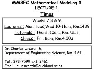
MM3FC Mathematical Modeling 3 LECTURE 6. Times Weeks 7,8 & 9. Lectures : Mon,Tues,Wed 10-11am, Rm.1439 Tutorials : Thurs, 10am, Rm. ULT. Clinics : Fri, 8am, Rm.4.503. Dr. Charles Unsworth, Department of Engineering Science, Rm. 4.611 Tel : 373-7599 ext. 8 2461

E N D
MM3FC Mathematical Modeling 3LECTURE 6 Times Weeks 7,8 & 9. Lectures : Mon,Tues,Wed 10-11am, Rm.1439 Tutorials : Thurs, 10am, Rm. ULT. Clinics : Fri, 8am, Rm.4.503 Dr. Charles Unsworth, Department of Engineering Science, Rm. 4.611 Tel : 373-7599 ext. 82461 Email : c.unsworth@auckland.ac.nz
This LectureWhat are we going to cover & Why ? • The Z-Transform. • (Makes convolution easy) • Cascading systems with the z-transform. • (simplifies the whole process)
The Z-Transform • We will now introduce the z-transform for FIR filters and finite length sequences in general. • We will use the FIR case to introduce the important concept of ‘domains of representation’. • We will learn that the z-transform brings polynomials and rational functions into the analysis of discrete time systems. • We will show that convolution is equivalent to polynomial multiplication and that common algebraic operations, such as multiplying, dividing and factoring polynomials can be interpreted as combining or decomposing LTI systems.
Definition of the Z-Transform • A finite length signal x[n] can be represented as : • And the conventional z-transform of such a signal is given by : Where, z represents any complex number. • All we are doing is ‘transforming’ the data x[n] into another representation X[z] to make the system easier to solve. • We say we are performing the ‘z-transform of x[n]’. … (5.1)
It is instructive to note, though, that X[z] can be re-written as : • This emphasizes that the variable (z-1) is a polynomial of degree k=N. • There is nothing complicated about performing a transform. • All we do to obtain X(z) is to construct a polynomial whose coefficients are the values of the sequence x[n] • Example 1 : Let’s determine the z-transform of our finite-sequence . • n n<-1 -1 0 1 2 3 4 5 n>5 • x[n] 0 0 2 4 6 4 2 0 0 • The z-transform is : X (z) = 2 + 4z-1 + 6z-2 + 4z-3 + 2z-4 … (5.2)
Example 2 : • Determine the sequence x[n] from the z-transform X(z). • X(z) = 1 –2z-1 + 3z-3 – z-5 • n n<-1 -1 0 1 2 3 4 5 n>5 • x[n] • You have just performed what is known as the ‘Inverse z-transform’. • Similarly, we can recover x[n] from X(z) by extracting the co-efficient values of X(z) and placing them in their corresponding kth position in the sequence x[n].
Domains • In general, a ‘z-transform pair’ is a sequence and it’s corresponding z-transform. n – Domain (or Time-Domain) z – Domain • Notice how (n) is the independent variable of the sequence x[n]. • Here, we say the signal exists in the ‘n-Domain’. • Since, (n) is often an index that counts time, we also say this is the ‘time-Domain’ of the signal. • Similarly, (z) is the independent variable of the z-transform X(z). • Thus, we the signal exists in the ‘z-Domain’. • During a ‘z-transform’ we move from the ‘time-Domain’ ‘z-Domain’. • In an ‘Inverse transform’ we move from the ‘z-Domain’ ‘time-Domain’. … (5.3)
Z-Transform of an Impulse • A simple but very important example is the z-transform pair of an impulse of a sequence x[n]. • As we know this can be defined as : x[n] =[n- n0] The co-efficient of the polynomial z-1 = magnitude of the impulse = 1. The kth power of the polynomial z-1 = the offset of the impulse = n0. n – Domain z – Domain • Now we’ve learned how to transform a signal from the n-Domain to the z-Domain …… but why ? …… • Next, we are going to answer this very question …… … (5.4)
( ) The z-transform & Linear Systems • The z-transform is indispensable in the design of LTI systems. • The reason is the way an LTI system responds to a particular input signal x[n] = zn for - n . Recall, the general difference equation of an FIR filter : … (5.5) The ‘system function’ of the FIR
We can see that the ‘system function’ of the FIR is a polynomial whose form depends on the coefficients of the FIR. • Thus, we define the ‘system function’ of an FIR filter to be : • The ‘system function’ is also the z-transform of the ‘impulse response’. • Thus, FIR filters with an input x[n] = zn for - n give an output y[n]. • y[n] = h[n] * zn = H(z)zn … (5.6) … (5.7) … (5.8)
Example 3 : Find the system function H(z) of the FIR filter with impulse response. h[n] = [n-1] – 7 [n-2] – 3 [n-3] Simply, replace the (n-k)’s with the corresponding z-k. Gives : H(z) = z-1 –7z-2 –3z-3 Example 4 : Find the impulse response h[n] of the FIR filter whose system response is. H(z) = 4(1 – z-1)(1 + z-1)(1 + 8z-1).
Properties of the z-transform … (6.9) • LINEARITY : The z-transform obeys the ‘principle of superposition’ or ‘linearity’ ax1[n] + bx2[n] aX1(z) + bX2(z) Example 5 : Calculate the linear superposition of the z-transforms of the two signals below. For a=1, b=1 x1[n] = [n] + [n-1] + 2 [n-2] + 3 [n-5] n -2 -1 0 1 2 3 4 5 x2 -2 3 -4 2 1 0 0 -2
Time Delay Property : The z-transform of a signal x[n] delayed by (n0) samples is equivalent to z-transform X(z) of x[n] mutiplied by z-n. • A delay of 1 sample multiplies the z-transform by z-1 • x[n-1] z-1X(z) • A delay of n0 samples multiplies the z-transform by z-n0 • x[n – n0] z-n0X(z) • Example 6 : The signal x1[n] = [n] + [n-1] + 2 [n-2] + 3 [n-5] is delayed by 6 time samples. Calculate its z-transform … (6.10)
The General z-Transform Formula • So far we have defined the z-transform H(z) only for finite input sequences x[n]. • The z-transform extends for infinite-length signals too. … (6.11)
x[n] x[n-1] Unit delay x[n]H(z) = x[n-1] x[n] z-1 The z-Transform in Block Diagrams • As we have seen a ‘unit delay’ becomes a z-1 operator in the z-Domain. • Similarly in a block diagram, all delays can be replaced by a z-n0 operator. = Equivalent Systems Example 7 : Draw a block diagram for the system: y[n] = (1 – z-1)x[n]
( ) Convolution & the z-Transform • Convolution in the ‘n-domain’ is multiplication in the ‘z-Domain’. = system function = H(z)
Convolution in the ‘n-Domain is multiplication in the z-Domain. y[n] = h[n] * x[n] y(z) = H(z)X(z) Example 8 : The signal x[n] = [n-1] –[n-2] + [n-3] – [n-4] is passed through the filter y[n] = x[n] – x[n-1]. Determine the output from the filter using convolution time-domain and the z-domain. In the Time-Domain … (4.12) n n< 1 1 2 3 4 5 n>4 x[n] 0 1 -1 1 -1 0 0 h[n] 1 -1 h[0] 0 1 -1 1 -1 0 0 h[1] 0 -1 1 -1 1 0 y[n] 0 1 -2 2 -2 1 0 y[n] = [n-1] –2[n-2] + 2[n-3] – 2[n-4] + 5[n-5]
For the z-Domain, express the signal & filter in terms of z’s and multiply. Then inverse transform to get the signal. (Just replace the z’s with ’s). Y[N] = X[N]*H[N] = (z-1 – z-2 + z-3 – z-4 )(1 – z-1) = z-1 – 2z-2 + 2z-3 – 2z-4 + z-5 y[n] = [n-1] –2[n-2] + 2[n-3] – 2[n-4] + 5[n-5] Transforming to the z-Domain is a simpler way to solve the system. Convolution in the z-Domain is just algebraic multiplication.
h1[n] h[n] = h1[n] * h2[n] [n] LTI 1 h1[n] LTI 2 h2[n] H2(z) H(z) = H1(z) H2(z) H1(z) Cascading Systems with the z-Transform • One of the main applications of the z-transform is in system design. • Remember, the impulse response of a 2 cascaded LTI systems. • We can now use the z-transform to determine the same thing. The system function for a cascade of 2 LTI systems is the product of the individual system functions. h[n] = h1[n] * h2[n] H(z) = H1(z)H2(z) • The z-transform, like convolution, is commutative so the LTI systems could be cascaded in either order. • As we can see, the formula would extend for (N) cascaded LTI systems. … (4.13)
x[n] x[n-1] z-1 3 -1 w[n] w[n-1] z-1 2 -1 y[n] Example 9 : Use the z-transform to cascade the two systems below and determine their combined difference equation. Draw the block diagram of the 2 cascaded system and its equivalent system. Which is the faster system ? w[n] = 3x[n] - x[n-1] ; y[n] = 2w[n] – w[n-1] Block diagram (here we see x[n] is the input to w[n] which inputs to y[n].) 2 cascaded 1st order systems. Order = power of highest z.
Just change to z’s and multiply out. The system functions are : • W(z) = 3 - z-1 and Y(z) = 2 –z-1 • Combined system function A(z) = W(z)Y(z) • A(z) = (3 - z-1)(2 –z-1) = 6 – 3z-1 – 2z-1 + z-2 • = 6 – 5z-1 + z-2 • Thus, a[n] = 6x[n] – 5x[n-1] + x[n-2] • Equivalent circuit. • The equivalent circuit is faster. 3 multipliers & 2 adders compared to the cascaded systems 4 multipliers and 2 adders. x[n] x[n-1] x[n-2] z-1 z-1 6 -5 1 a[n] A 2nd order system
Example 10 : Use z-transform to combine the following cascaded systems. Again draw the block diagram of the 2 cascaded system and its equivalent system. What are the orders of the systems ? Which is the faster system ? w[n] = x[n] + x[n-1] and y[n] = w[n] – w[n-1] + w[n-2]
w[n] y[n] x[n] LTI 1 LTI 2 H2(z) = 1 - z-1 + z-2 H1(z) = z-1 – 1 Factoring z-Polynomials • If we can multiply z-transforms to get higher-order systems we can also factorise z-polynomials to break down a large system into smaller modules. Example : Consider H(z) = 1 –2z-1 + 2z-2 – z-3 First we visually inspect for roots that may exist. We can see one root at z = 1. Therefore, (z-1 – 1) is a factor. Now, H(z) = H1(z)H2(z) Therefore, H2(z) = H(z)/H1(z) = (1 –2z-1 + 2z-2 – z-3)/ (z-1 – 1) = 1 - z-1 + z-2 • Thus, the 3rd order LTI can be factorised into a cascaded 1st & 2nd order system.
Deconvolution (Inverse filtering) • The cascading property leads to the question …… • “ Can we use the 2nd filter in cascade to undo the effect of the 1st filter” ? • If H1(z) is known then we can construct a filter H2(z) to undo the effect of the first by setting H(z) = 1. H(z) = H1(z)H2(z) = 1 Thus, H2(z) = 1/H1(z) • The 2nd filter tries to ‘undo the convolution’ that exists, so the process is referred to as ‘deconvolution’. • The process is also called ‘Inverse Filtering’. Example : Determine the inverse filter for H1(z) = 1 – z-1 + ½z-2. Now, H1(z)H2(z) = 1
Thus, H2(z) = 1/ 1 – z-1 + ½z-2 • What are we to make of this example ? • It seems that the inverse filter for an FIR filter must have a system function that is not a polynomial. • Instead, the inverse filter is a rational function (ratio of 2 polynomials). • Thus, the inverse filter cannot be an FIR filter. • And Deconvolution is not as simple as it appeared ! • Later, we will learn about other LTI systems that do have rational system functions and will return to the problem of deconvolution.