Download
1 / 41
410 likes | 532 Views
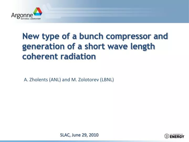
New type of a bunch compressor and generation of a short wave length coherent radiation. A. Zholents (ANL) and M. Zolotorev (LBNL). SLAC, June 29, 2010. DE/E. D E/E. s z 0. ‘chirp’. z. z. s E / E. D z = R 56 D E/E. V = V 0 sin( wt ). RF Accelerating Voltage. Path Length-Energy

E N D
New type of a bunch compressor and generation of a short wave length coherent radiation A. Zholents (ANL) and M. Zolotorev (LBNL) SLAC, June 29, 2010
DE/E DE/E sz0 ‘chirp’ z z sE/E Dz = R56DE/E V = V0sin(wt) RF Accelerating Voltage Path Length-Energy Dependent Beamline Magnetic Bunch Compression Courtesy P. Emma DE/E under-compression z sz Chicane RF
“Any fool with four dipoles can compress a bunch” - anonymous OK, but there may be a few details to consider… P. Emma, ICFA Workshop, Sardinia, 2002
DE/E z sz Full compression is not good because of emittance growth due to CSR LCLS Full compression under-compression K. Bane et al., PRST AB, 12, 030704 (2009) Some issues DE/E Needs: de-chirping De-chirping is typically done by using wake fields and/or off-crest acceleration under-compression z sz
References Results presented here use the idea of transverse to longitudinal emittance exchange M. Cornacchia, P. Emma, “Transverse to longitudinal emittance exchange”, Phys. Rev. ST Accel. Beams 5, 084001 (2002) P. Emma, Z. Huang, K.-J. Kim, P. Piot, “Transverse-to-Longitudinal Emittance Exchange to Improve Performance of High-Gain Free-Electron Lasers”, Phys. Rev. ST Accel. Beams 9, 100702 (2006). R.P. Fliller, D.A. Edwards, H.T. Edwards, T. Koeth, K.T. Harkay, K.-J. Kim, “Transverse to longitudinal emittance exchange beamline at the A0 Photoinjector”, Part. Acc. Conf., PAC07, (2007).
Variant 1 M+ D+ M+ T M- D- M- QD QF QD QF QD QF QD QF QD B B QF QF QD B B B B QF QD QD QF B B TM110 TM010 TM010 Deflecting cavity A schematic of the bunch compressor (manipulate longitudinal phase space with ease of a transverse phase space) Focusing properties of individual sections I I I T I QD QF QD QF QD QF QD QF B B QD QF QF QD B B B B QF QD QD QF z →x emit. exch. x → z emit. exch. Telescope B B
M+ D+ M+ B B QD QD QF QD QF QD QF QF QF QD QD B B B QF QF QD QD TM110 TM010 TM010 B B Deflecting cavity Variant 2 M+ D+ M+ T B A schematic of the bunch compressor: alternative variant
Deflecting cavity B B Courtesy: Li, Corlett Thin cavity approximation: In agreement with Panofsky-Wentzel theorem
Thick deflecting cavity: d1 TM110 One can cancel unwanted energy gain using two TM010 mode side cavities d TM010 TM110 TM010 Required energy gain in each TM010 cavity
FNAL: SRF five cell prototype Ebeam = 250 MeV fRF= 3.9 GHz V0 = 4 MV (1m, 3x7 cells: Li, Corlett) V1 = 0.4 MV k = 0.013 cm-1 SLAC: copper X-band LOLA Ebeam = 250 MeV fRF= 11.4 GHz V0 = 22 MV ( 0.5 m) V1 = 6.6 MV k = 0.21 cm-1
Input Coupler HOM Damper LOM Damper HOM Dampers Single-Cell SC Cavity Total length = 128 mm Voltage gap = 53 mm Courtesy G. Waldschmidt
First leg of emittance exchange scheme B QF QD B Complete emittance exchange scheme QD QF QD B B QF QD B The following constrains were used:
T QD QF QD QF QD QF I I I T I QD QF QD QF QD QF QD QF QD B B QF QF QD B B B B QF QD QD QF z →x emit. exch. x → z emit. exch. Telescope B B Telescope Total transformation
Define: - bunch length before compression, - uncorrelated relative energy spread before compression, and - energy chirp before compression - bunch length after compression, - uncorrelated relative energy spread after compression Bunch length and energy spread at the end of the scheme Using entire mapping one obtains :
No chirp case, e.g., h = 0 Case 1 then Case 2 Then the compression is not yet finished
The last element of proposed BC is the chicane/dogleg with its R56 used to cancel the R56 accumulated upstream Then, the entire mapping takes the following form: … and we obtain for the final bunch length and relative energy spread:
… or one may prefer to wait until the electron beam gains energy from E1 to E2 and do the final compression at E2 Then R56 for the final step should be: … and we obtain for the final bunch length and relative energy spread: Possible advantage of aDeferred Compression is reduction of the gain of the microbunching instability and impact of other collective forces: a) electron bunch is not yet compressed to the shortest size b) energy spread has already grown up to the final value
Possible advantages • Because there is no need in energy chirp for compression: • one can use BC even after the linac and obtain final compression in a “spreader”/ “dogleg” part of the lattice leading to FEL Gun L1 Spreader L2 BC BC b) or use two BCs, one in usual location and one after the linac
Possible advantages (2) Accelerate a relatively long bunch in the re-circulating linac without a chirp and compress it in the final arc. FEL New type of a bunch compressor Possible cost saving
Jitter studies No adverse jitter effects are found in a linear approximation. Timing jitter is compressed by a compression factor and energy jitter is increased by a compression factor When exact cavity fields with Bessel, Sin and Cos functions were considered the following results were obtained: Coordinate jitter after compression driven by the energy jitter before compression: Main parameters: 1 – precise calculation 2 – estimation using expression: • frf = 12 GHz • h=40 cm • m=20 • = 10 cm Lcav = 100 cm Formula can be understood via Taylor expansion of the following expression:
1) h = 20 cm, 2) h = 40 cm 1) h = 20 cm, 2) h = 40 cm Same as before, but for 3 GHz rf and two sets of dispersion function: Main parameters: • frf = 3 GHz • m=20 • = 10 cm Lcav = 100 cm Same as before, but now for an angular jitter
Energy jitter shows ordinary increase due to compression with m=20 1) h = 20 cm, 2) h = 40 cm Practically no timing jitter due to energy jitter
Timing jitter shows ordinary decrease due to compression with m=20 Practically no coordinate jitter due to timing jitter
Practically no energy jitter due to coordinate jitter Practically no timing jitter due to coordinate jitter
Practically no timing jitter due to angular jitter Practically no energy jitter due to angular jitter
Reduction of the coordinate jitter driven by energy jitter Second rf cavity is set approximately at 0.5% high value to reduce jitter in x. Conditions k1h1=-1 and k2h2=-1 are observed. 1) h1 = 20 cm, 2) h1 = 40 cm 1) h1 = 20 cm, 2) h1 = 40 cm
Illustration In the following numerical example we use: fRF = 2.85 GHz k=0.05 cm-1 cavity length = 1 m At Eb = 250 MeV this corresponds to: V0 = 21 MV V1 = -8.7 MV
Illustration: compression by a factor of 15 -I -I -I -I T B1 tcav tcav B2 B2 B1 B2 B2 Magnets: jB1= 0.10 jB2= 0.0445 Length=0.3 m bx=0.25 m bx=56 m Lattice functions for a bunch compressor with a telescopic factor m=15. Note, matching of the vertical beta-function was not pursued.
QD 5 7 1 8 3 4 6 2 QF QD QF QD QF QD QF QD B B QF QF QD B B B B QF QD QD QF B B Numerical values of beam sizes at key locations Deferred compression 42 mm -> 10 mm m=15 Input parameters Eb=250 MeV ex=0.5 mm sd0=10-4 sE0=25 keV sz0= 160 mm
Same as before, but with a reduced energy spread to 5 keV m=15 Eb=250 MeV ex=0.5 mm sd0=2x10⁻⁵ sE0=5 keV sz0= 160 mm
Same as before, but with a reduced beam energy to 100 MeV This may eliminate a need in the laser heater m=15 Eb=100 MeV ex=0.5 mm sd0=5x10⁻⁵ sE0=5 keV sz0= 160 mm
Same as before, but with increased bunch length to 640 mm m=15 Eb=100 MeV ex=0.5 mm sd0=5x10⁻⁵ sE0=5 keV sz0= 640 mm
px assume: Dpx=spx/100 z Eb=100 MeV Emittance degradation DE z x Concern: space charge induced energy modulation in the telescope section can transfer into the coordinate space and be seen as emittance degradation z Eb=250 MeV • ex = 0.5 mm • sE0 =5 keV • sz0= 160 mm • h = 0.25 m • 0= 0.25 m • b1= 10 m Inside telescope Ipeak=3 kA No emittance degradation is expected
Compression of the laser induced energy modulation for microbunching at a shorter wave length Compression factor, m=20 laser BC Laser e-beam interaction Initial modulation DE/sE DE/sE Compressed modulation z/l z/l Bunching efficiency at m-th harmonic of modulating frequency: DE/sE HGHG: EEHG: This method: z/l Plots of longitudinal phase space at various locations
DE/sE … or be deferred to a “spreader”/“dogleg” z/l BC Laser e-beam interaction Linac Spreader Compression of the laser induced energy modulation can also be made at the end of the linac BC Laser e-beam interaction Linac
Compression of the Echo induced microbunching BC Compression factor, m=5 DE/sE z/l z/l
zoom on one peak z/l Compression of the Echo induced microbunching (2) Peak current after compression, kA 1 0.8 0.6 0.4 0.2 z/l
Producing 1 nm seeding beginning from 200 nm laser modulation Echo: harmonic number = 20 new type BC, m=10 traditional BC Gun L1 L2 Echo Spreader BC BC Ipeak=100 A Ipeak=1 kA Total harmonic number = 20x10 = 200 !
Other uses It is often desirable to get rid off the tails in longitudinal distribution and proposed scheme can be used as efficient tail cutter collimator QD QF QD QF QD QF QD QF QD B B QF QF QD B B B B QF QD QD QF x → z emit. exch. z →x emit. exch. FODO B B
Other uses (3) Longitudinal phase space tomography x- px tomography here is d- ztomography there QD QF QD QF QD QF QD QF QD B B QF QF QD B B B B QF QD QD QF x → z emit. exch. z →x emit. exch. Telescope B B
Summary • Efficient electron bunch manipulation in the longitudinal phase space can be accomplished by first exchanging longitudinal and transverse emittances, manipulating electrons in the transverse phase space and finally exchanging emittances back to their original state. • One application is bunch compressor that does not need energy chirp • This can also be used for a compression of any features introduced to the electron bunch, like, for example energy modulation produced in interaction with the laser. • Proposed techniques for a bunch compression allows deferred compression that might be useful to mitigate possible adverse effects caused by collective forces.