Download
1 / 33
330 likes | 354 Views
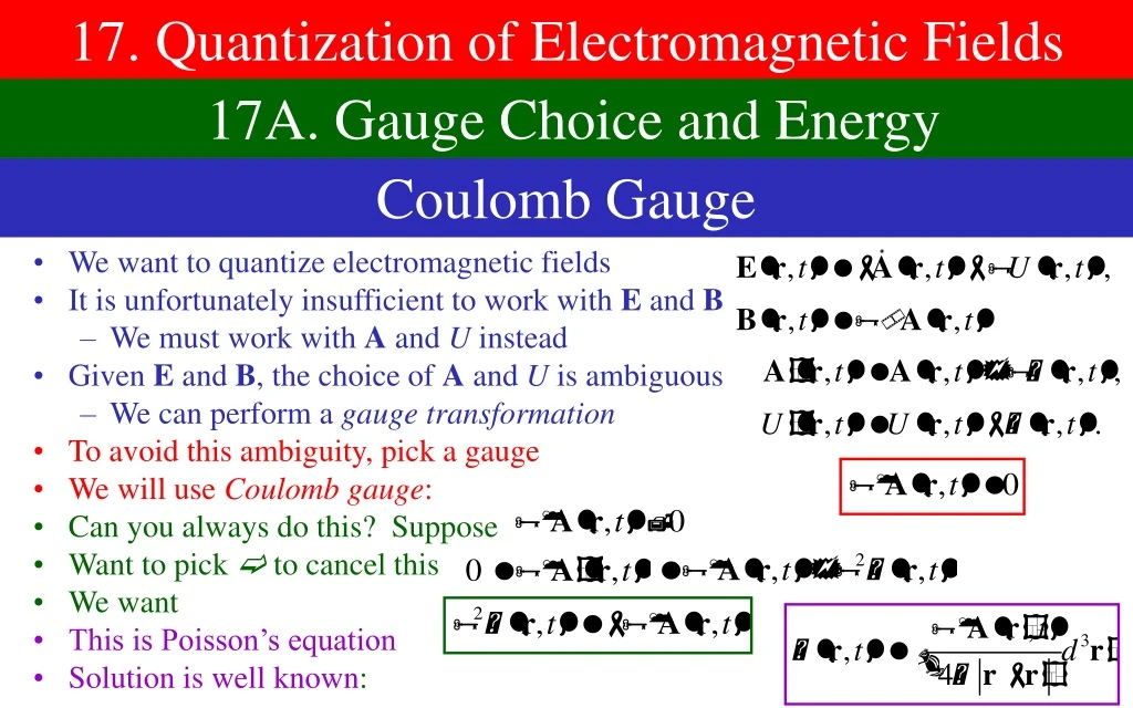
17. Quantization of Electromagnetic Fields. 17A. Gauge Choice and Energy. Coulomb Gauge. We want to quantize electromagnetic fields It is unfortunately insufficient to work with E and B We must work with A and U instead Given E and B , the choice of A and U is ambiguous

E N D
17. Quantization of Electromagnetic Fields 17A. Gauge Choice and Energy Coulomb Gauge • We want to quantize electromagnetic fields • It is unfortunately insufficient to work with E and B • We must work with A and U instead • Given E and B, the choice of A and U is ambiguous • We can perform a gauge transformation • To avoid this ambiguity, pick a gauge • We will use Coulomb gauge: • Can you always do this? Suppose • Want to pick to cancel this • We want • This is Poisson’s equation • Solution is well known:
Working With Coulomb Gauge • In Coulomb gauge, we can find the electric potential U(r,t) • This is Poisson equation again • In the absence of sources, U = 0 Energy Density and Energy • Energy density of EM fields: • Use the fact that c2 = 1/(00): • Integrate to get the total energy:
17B. Fourier Modes and Polarization Vectors Finite Volume and Fourier Modes • Although it isn’t obvious, this is justa lot of coupled Harmonic oscillators • The curl terms just couple A(r) to “adjacent” values of r • As an aid to thinking about things, we will pretend theuniverse has volume V = L3, with periodic boundary conditions • Later we will take L • Periodic boundary conditions means that any function repeatsif you go a distance L in any direction • To decouple modes, write A(r,t) in terms of Fourier modes • Because of periodic boundary condi-tions, k is restricted to certain values:
Writing the Energy in Fourier Modes: • We now substitute this into the expression for E: • Then for example,the x-integral yields • Integral is only non-zero if k + k'= 0 • This lets us do integrals and one sum:
Some Restrictions on A: • We must make sure A(r,t) is real: • Effectively, there are only half as many Ak’s as you think there are • We are also workingin Coulomb gauge: • Use these expressionsto simplify E: • We have some redundancies in the sum • Because Ak and A–k are related • To avoid redundancy, arbitrarily pick half of the k’s to be positive • Rewrite sums overjust half of the k’s
Polarizations: • Ak actually has only two components • Choose two unit vectors k for = 1,2, the polarization vectors, such that: • Usually pick them real, but you don’t have to • Then any vector Ak perpendicular to k can be written: • Our energy is now:
17C. Quantizing the Electromagnetic Fields Comparison to Complex Harmonic Oscillator • Compare to the complex harmonic oscillator: • This is just a sum of complex harmonic oscillators! • We need the analogous relations: • Old formulas: • New formulas:
Simplifying the Notation • The a’s have commutation relations: • All other commutators vanish • Keep in mind, we have restricted k’s to half of the values, just k > 0 • Unnecessarily complicated, since we have k label and label • Easier to combine this to a single notation • Now commutation relations: • All others vanish • The expressionsabove thensimplify, slightly
Vector Potential as an Operator • We want to write out A in terms of a’s: • Not manifestly Hermitian • Can be fixed by redoing second term in sum with k –k • Also, some complicated details of how we specified modes demands • We therefore have:
Electric and Magnetic Field Operators • To get magnetic field, just use • For electric field, we use • As before, on last term, let k –k • Note all fields are functions ofposition r, but no longer time t
Comments on Field Operators • Note that time dependence isnow gone • All fields are now operators Compare to ordinary quantum: • Position and momentumare classically functionsof time, x(t) and p(t) • When you quantize it, theybecome operators X and P • Any time dependence will be in the state vector |(t) • Just like any other operator, field operators A(r), etc., will be uncertain • You can measure things like E(r) and B(r) • You can’t measure A(r) because it’s not gauge invariant • We have an infinite number of operators • Which makes describing quantum states |(t) hard
17D. Eigenstates of the Electromagnetic Field Subtracting Infinity from the Energy • Our Hamiltonian is a sum of harmonic oscillators • Ground state we will call |0; it has the property for all k and • Problem: the energy of this state is infinite: • This infinity persists even if youdivide by the volume V of the universe • Solution – you can always add a constant to the Hamiltonian • Energy for all states is now finite • These infinities come up repeatedly in quantum field theory • They are generally dealt with by a process called renormalization • This one is the easiest to deal with
Labeling General Eigenstates • Normally give eigenvalues of all number operators • This would be an infinitely long list • Most of these states would have infinite energy To avoid this problem: • List only states that are non-zero: • You have n1 photons with wave number k1 and spin 1, etc. • Any terms with ni= 0 is irrelevant • Since it’s just a list,order doesn’t matter • Energy of this state is: • State can be constructed from the vacuum state as
Abbreviations and Notation • Sometimes understood that you onlyhave one photon of a given type. Drop ni: • Do we ever write wave functions?No! You will go insane! Need to get good at how raising and lowering operators affect things: • Lowering operator decreasesnumberof photons present ifthat photon is present to begin with: • Raising operator creates aphoton whether one waspresentor not: • Whenever possible, try to keep expressions simple; lower first
Sample Problem An electromagnetic system at t = 0 is in the state , where and . (a) Find the state vector at all times (b) Find the expectation value of the electric field at all times • General solution to Schrödinger’s equation is: • The two portions of (0) givenare both eigenvectors of H • Each of these terms will just pick up a phase • Electric field operator is: • So we want:
Sample Problem (2) (b) Find the expectation value of the electric field at all times • We must either increase the number of photons by one, or decrease it by one • The only terms that matter are therefore:
Sample Problem (3) (b) Find the expectation value of the electric field at all times • Use some simple identities:
17E. Momentum of Quantum States Begin the Calculation • We have been talking as if we have particles (“photons”) with energy • To cement this concept, let’s find the momentum • We first need the momentum density from E & M: • Integrate it over space to get the momentum: • Recall our expressions for E and B: • Substitute them into Pem:
Integrals and One Sum are Easy • The integrals we have seen before: • Substitute this in. Note that the k’s automatically will cancel • Do thesum on k' • Expand the tripleproducts. Use thatkis perpendicularto k:
More Stuff Goes Away On first and last term: • Note that if you take k –k, and exchange ' the expressions would be identical • Because all k is summed over, and and ' are summed over, this means there is an identical cancelling sum somewhere in the expression • Recall our polarization vectors are orthonormal • This makes the ' sum easy: • Commutation relationsallow us to rewrite • Our penultimate form:
Answer and Interpretation: • On the last term, positive values ofk will be cancelled by negative values • Eigenstates of H will have momentum: • Clearly, each photon has momentum p = k • Since the energy was , and = ck, this tells us E = cp • Correct for relativistic particles
17F. Taking the Infinite Volume Limit • We said we were going to take L3 = V , but how do we do this? • First step: Consider the following integral • We know how to do this inboth finite and infinite volume • So we have: • Second step: Consider an integral over k in one dimension • Recall how this is defined • Remember that our k’s are discrete: • So we have • Therefore, in 1D: • In three dimensionsthis becomes:
17G. The Nature of the Vacuum Things Are Not As Simple As They Seem • What is the value of the electric or magnetic field for the vacuum state |0? • These fields are operators, so like other operators, expect them to have a distribution • With an expectation value and an uncertainty • Let’s find expectation value and uncertainty • Let them act on the vacuum state • The annihilation terms vanish • The creation terms create one-particle states
So We Find: • It is trivial to see that: • On the other hand, the expectation value of the square of E is: • Take limit V : • Similar computation for magnetic field:
Interpretation • It is easy to see that both of these integrals diverge • Implies there should be infinite random electric fields, even for empty space • How come we don’t notice this? • All probes of electric or magnetic field are in fact finite in extent • Even though we think we are measuringE(r), we are actually measuring • The “aperture function” f(s) tells how the measurement is spread over space • Normalized to 1 • The function fsmooths out E, suppressing high momentum modes • Effectively cuts off integrals over k • This will lead to finite values:
Sample Problem The electric field of the vacuum is measured using the aperture function: Find the expectation values for Ef(r) and Ef2(r). • We first find • So we need
Sample Problem (2) The electric field of the vacuum is measured using the aperture function: Find the expectation values for Ef(r) and Ef2(r). • It is obviousthat as usual: • For Ef2(r): • Take limit V , then let a2k2 = x
17H. The Casimir Effect Can We Really Ignore the Infinite Energy? • We found the expectationvalue of E2 and B2: • Energy densityexpectation value is then • This is the same infinity as the infinity we discarded in H • As Sidney Coleman of Harvard used to say:“Just because something is infinite doesn’t mean it’s zero!” • Though it is unlikely any measurement will ever yield infinity, maybe this will contribute if we change the Hamiltonian
Modes in a Capacitor • Consider a parallel plate capacitor • Area L2, separation a • Assume L >> a • E|| must vanish at the conducting surface • We can get the modes to vanish on theboundaries z = 0 and z = a if we use modes • nx = 0, 1, 2, … • nz = 0, 1, 2, … • We still need kAk= 0 • This means there will be two polarization modes • We can also get modes with E||= 0 by choosing • We still need kAk= 0 • To get it E||= 0 on the boundary • Which we can arrange by picking Akin the z-direction • Which means there is only one mode L L a
Energy in a Capacitor • Each mode contributes an energy • Total energy forseparation ais therefore • For kxand ky, we can take the limit L using the usual rule • The energy density in the absence of the capacitor is • So in the energy in thissame volume would be • Maybe we can find thedifference in energy • Problem – this is infinity minus infinity L L a
Regulating the Sum • These sums/integrals are both infinite • Physically, at very high frequency, allconductorsbecome transparent anyway • Add a regulator function that cuts off integrals at infinity • Can show the form of the regulator doesn’t make much difference • We will pick the cutoff function e–k L L a
Do Some Sums • Sum on polarizations,and substitute for kz: • Some sum theorems: • We therefore have: • Write interms of • Cutoff frequency will be high, so w will be small
Take the Limit and Interpret • Expand in the limit of small w • Let Maple can do it for us • Note that the energy is negative • Capacitor plates prefer to be near each other • Take derivative to get a force • Note this is force per unit area, or pressure • Negative pressure, since it attracts • Experimentally observed L L a