Download
1 / 9
90 likes | 215 Views
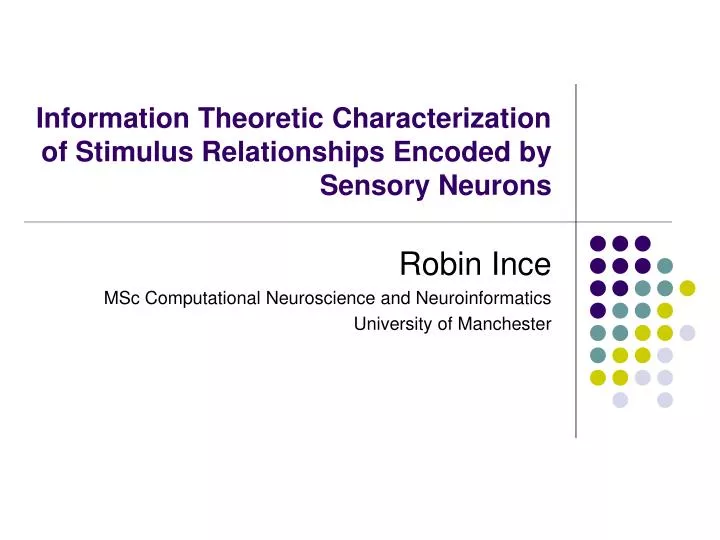
Information Theoretic Characterization of Stimulus Relationships Encoded by Sensory Neurons. Robin Ince MSc Computational Neuroscience and Neuroinformatics University of Manchester. Output (spike or no spike). Inputs (stimulus features). Black Box System (neuron). Introduction.

E N D
Information Theoretic Characterization of Stimulus Relationships Encoded by Sensory Neurons Robin Ince MSc Computational Neuroscience and Neuroinformatics University of Manchester
Output (spike or no spike) Inputs (stimulus features) Black Box System (neuron) Introduction
Subspace of distributions with no higher order interactions Subset of distributions sharing same pairwise marginals True Distribution Projection of true distribution: Maximum Entropy Solution Maximum Entropy Method • a principled way to investigate interactions • same marginals as true distribution but no higher order effects • solution via Information Geometry (Amari, 2001)
Information Decomposition I(k;R) = IS(2)(k) + I(1)(k;R) + I(=2)(k;R) + IHO(k;R) • IS(2)(k) = H(k) – H(2)(k) • I(1)(k;R) = H(1)(k) – H(1)(k|R) • I(=2)(k;R) = I(2)(k;R) – I(1)(k;R) = H(2)(k) – H(1)(k) + H(1)(k|R) – H(2)(k|R) • IHO(k;R) = H(2)(k|R) – H(k|R)
Output Features processed separately Conclusions • few underlying assumptions; widely applicable • accurate predictions; good temporal precision • can be difficult to interpret