Download
1 / 44
440 likes | 598 Views
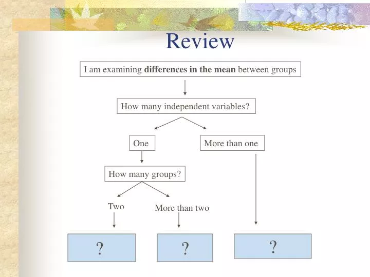
Review . I am examining differences in the mean between groups. How many independent variables? . One . More than one . How many groups?. Two . More than two . ? . ?. ?. Differences or Relationships? . I am examining relationships between variables.

E N D
Review I am examining differences in the mean between groups How many independent variables? One More than one How many groups? Two More than two ? ? ?
Differences or Relationships? I am examining relationships between variables I am examining differences between groups T-test, ANOVA Correlation, Regression Analysis
Example of Correlation Is there an association between: • Children’s IQ and Parents’ IQ • Degree of social trust and number of membership in voluntary association ? • Urban growth and air quality violations? • GRA funding and number of publication by Ph.D. students • Number of police patrol and number of crime • Grade on exam and time on exam
Correlation • Correlation coefficient: statistical index of the degree to which two variables are associated, or related. • We can determine whether one variable is related to another by seeing whether scores on the two variables covary---whether they vary together.
Scatterplot • The relationship between any two variables can be portrayed graphically on an x- and y- axis. • Each subject i1 has (x1, y1). When score s for an entire sample are plotted, the result is called scatter plot.
Direction of the relationship Variables can be positively or negatively correlated. • Positive correlation: A value of one variable increase, value of other variable increase. • Negative correlation: A value of one variable increase, value of other variable decrease.
Strength of the relationship The magnitude of correlation: • Indicated by its numerical value • ignoring the sign • expresses the strength of the linear relationship between the variables.
r =1.00 r = .42 r =.17 r =.85
Pearson’s correlation coefficient There are many kinds of correlation coefficients but the most commonly used measure of correlation is the Pearson’s correlation coefficient. (r) • The Pearson r range between -1 to +1. • Sign indicate the direction. • The numerical value indicates the strength. • Perfect correlation : -1 or 1 • No correlation: 0 • A correlation of zero indicates the value are not linearly related. • However, it is possible they are related in curvilinear fashion.
Standardized relationship • The Pearson r can be thought of as a standardized measure of the association between two variables. • That is, a correlation between two variables equal to .64 is the same strength of relationship as the correlation of .64 for two entirely different variables. • The metric by which we gauge associations is a standard metric. • Also, it turns out that correlation can be thought of as a relationship between two variables that have first been standardized or converted to z scores.
Correlation Represents a Linear Relationship • Correlation involves a linear relationship. • "Linear" refers to the fact that, when we graph our two variables, and there is a correlation, we get a line of points. • Correlation tells you how much two variables are linearly related, not necessarily how much they are related in general. • There are some cases that two variables may have a strong, or even perfect, relationship, yet the relationship is not at all linear. In these cases, the correlation coefficient might be zero.
Coefficient of Determination r2 • The percentage of shared variance is represented by the square of the correlation coefficient, r2 . • Variance indicates the amount of variability in a set of data. • If the two variables are correlated, that means that we can account for some of the variance in one variable by the other variable.
Statistical significance of r • A correlation coefficient calculated on a sample is statistically significant if it has a very probability of being zero in the population. • In other words, to test r for significance, we test the null hypothesis that, in the population the correlation is zero by computing a t statistic. • Ho: r = 0 • HA: r = 0
Some consideration in interpreting correlation 1. Correlation represents a linear relations. • Correlation tells you how much two variables are linearly related, not necessarily how much they are related in general. • There are some cases that two variables may have a strong perfect relationship but not linear. For example, there can be a curvilinear relationship.
Some consideration in interpreting correlation 2. Restricted range (Slide: Truncated) • Correlation can be deceiving if the full information about each of the variable is not available. A correlation between two variable is smaller if the range of one or both variables is truncated. • Because the full variation of one variables is not available, there is not enough information to see the two variables covary together.
Some consideration in interpreting correlation 3. Outliers • Outliers are scores that are so obviously deviant from the remainder of the data. • On-line outliers ---- artificially inflate the correlation coefficient. • Off-line outliers --- artificially deflate the correlation coefficient
On-line outlier • An outlier which falls near where the regression line would normally fall would necessarily increase the size of the correlation coefficient, as seen below. • r = .457
Off-line outliers • An outlier that falls some distance away from the original regression line would decrease the size of the correlation coefficient, as seen below: • r = .336
Correlation and Causation • Two things that go together may not necessarily mean that there is a causation. • One variable can be strongly related to another, yet not cause it. Correlation does not imply causality. • When there is a correlation between X and Y. • Does X cause Y or Y cause X, or both? • Or is there a third variable Z causing both X and Y , and therefore, X and Y are correlated?
Simple Linear Regression • One objective of simple linear regression is to predict a person’s score on a dependent variable from knowledge of their score on an independent variable. • It is also used to examine the degree of linear relationship between an independent variable and a dependent variable.
Example of Linear Regression • Predict “productivity” of factory workers based on the “Test of Assembly Speed” score. • Predict “GPA” of college students based on the “SAT” score. • Examine the linear relationship between “Blood cholesterol” and “fat intake”.
Prediction • A perfect correlation between two variables produces a line when plotted in a bivariate scatterplot • In this figure, every increase of the value of X is associated with an increase in Y without any exceptions. If we wanted to predict values of Y based on a certain value of X, we would have no problem in doing so with this figure. A value of 2 for X should be associated with a value of 10 on the Y variable, as indicated by this graph.
Error of Prediction: “Unexplained Variance” • Usually, prediction won't be so perfect. Most often, not all the points will fall perfectly on the line. There will be some error in the prediction. • For each value of X, we know the approximate value of Y but not the exact value.
Unexplained Variance • We can look at how much each point falls off the line by drawing a little line straight from the point to the line as shown below. • If we wanted to summarize how much error in prediction we had overall, we could sum up the distances (or deviations) represented by all those little lines. • The middle line is called the regression line.
The Regression Equation • The regression equation is simply a mathematical equation for a line. It is the equation that describes the regression line. In algebra, we represent the equation for a line with something like this: y = a + bx
Sum of Squares Residual • Summing up the deviations of the points gives us an overall idea of how much error in prediction there is. • Unfortunately, this method does not work very well. • If we choose a line that goes exactly through the middle of the points, about half of the points that fall off of the line should be below the line and about half should be above. Some of the deviations will be negative and some will be positive, and, thus the sum of all of them will equal 0.
Sum of Squares Residual • The (imaginary) scores that fall exactly on the regression line are called the predicted scores, and there is a predicted score for each value of X. The predicted scores are represented by y^ • (sometimes referred to as "y-hat", because of the little hat; or as "y-predict"). • So the sum of the squared deviations from the predicted scores is represented by
Sum of Square Residual • y scores is subtracted from the predicted score (or the line) and then squared. Then all the squared deviations are summed a measure of the residual variation • sum of the squared deviations from the regression line (or the predicted points) is a summary of the error up. • Notice that this is a type of variation. It is the unexplained variation in the prediction of y when x is used to predict the y scores. Some books refer to this as the "sum of squares residual" because it is of prediction
Regression Line • If we want to draw a line that is perfectly through the middle of the points, we would choose a line that had the squared deviations from the line. Actually, we would use the smallest squared deviations. This criterion for best line is called the "Least Squares" criterion or Ordinary Least Squares (OLS). • We use the least squares criterion to pick the regression line. The regression line is sometimes called the "line of best fit" because it is the line that fits best when drawn through the points. It is a line that minimizes the distance of the actual scores from the predicted scores.
No relationship vs. Strong relationship • The regression line is flat when there is no ability to predict whatsoever. • The regression line is sloped at an angle when there is a relationship.
Sum of Squares Regression: The Explained Variance • The extent to which the regression line is sloped represents the amount we can predict y scores based on x scores, and the extent to which the regression line is beneficial in predicting y scores over and above the mean of the y scores. • To represent this, we could look at how much the predicted points (which fall on the regression line) deviate from the mean. • This deviation is represented by the little vertical lines I've drawn in the figure below.
Formula for Sum of Squares Regression: Explained Variance • The squared deviations of the predicted scores from the mean score, or • represent the amount of variance explained in the y scores by the x scores.
Total Variation • The total variation in the y score is measured simply by the sum of the squared deviations of the y scores from the mean.
Total Variation • The explained sum of squares and unexplained sum of squares add up to equal the total sum of squares. The variation of the scores is either explained by x or not. Total sum of squares = explained sum of squares + unexplained sum of squares.
R2 • The amount of variation explained by the regression line in regression analysis is equal to the amount of shared variation between the X and Y variables in correlation.
R2 • We can create a ratio of the amount of variance explained (sum or squares regression, or SSR) relative to the overall variation of the y variable (sum of squares total, or SST) which will give us r-square.
Multiple Regression • Multiple regression is an extension of a simple linear regression. • In multiple regression, a dependent variable is predicted by more than one independent variable • Y = a + b1x1 + b2x2 + . . . + bkxk