Download
1 / 20
200 likes | 279 Views
Nicholas Shields SESI Presentation – CUA Student Brian Dennis (Mentor). Frequency Distribution of GOES Solar Flare Peak Fluxes from 1994 to 2005. OVERVIEW. Background on GOES satellites GOES Event list Size Distribution Fit power-law to the size distribution. What is GOES?.

E N D
Nicholas Shields SESI Presentation – CUA Student Brian Dennis (Mentor) Frequency Distribution of GOES Solar Flare Peak Fluxes from 1994 to 2005
OVERVIEW • Background on GOES satellites • GOES Event list • Size Distribution • Fit power-law to the size distribution
What is GOES? • Geostationary Operational Environmental Satellites • X-ray Spectrometer • 3 second data in two wavelengths • 1-8 Angstrom • 0.5-4 Angstrom
Event Detection • First we take the raw data and smooth it using either a boxcar smoothing or an average smoothing • The derivative of the data is taken • Where the derivative crosses zero we find either a peak or a valley
Data-drop/spike Filter: • The SDAC data often has drops or spikes that we do not want to declare peaks and valleys.
Time Filter • The time intervals between a valley the next peak and the following valley are examined:
Quantization Filter • Quantization level = flux value where the step size changes • Matches peak flux to quantization level • Difference between peak and valley flux values must be greater than quantization step * 3
Background Subtraction: Method • GOES satellite records even non-flaring plasma • Difficult to distinguish the flux levels of the smaller solar flares • Linear background subtraction • Runs from one valley to the next • It takes the flux level at the first valley and subtracts it from every point in the data array until reaching the next valley
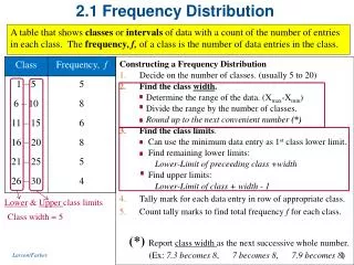
Size Distribution • A size distribution was performed on • un-subtracteddata • background subtracted data. • Binned the data by the flare size • Shows the frequency of solar flares over time based on their size
Power-Law Fits • Used OSPEX (object spectral executive) • Automatic fit using the closest parameter settings • Single power law fit • dN(p)/dp = A p−α • dN(p) is the number of events with a “size” between p and p + dp • A is a normalization parameter • and α is the power-law index
Work Still to be Done: • Change to creating a size distribution for a set number of flares rather than a set time interval • Use c-statistic to find the fit parameters rather than chi-squared
Acknowledgements • Brian Dennis • Andy Gopie • Richard Schwartz • Kim Tolbert • Fred Bruhweiler