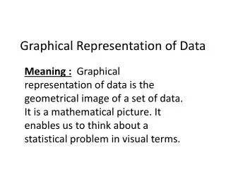
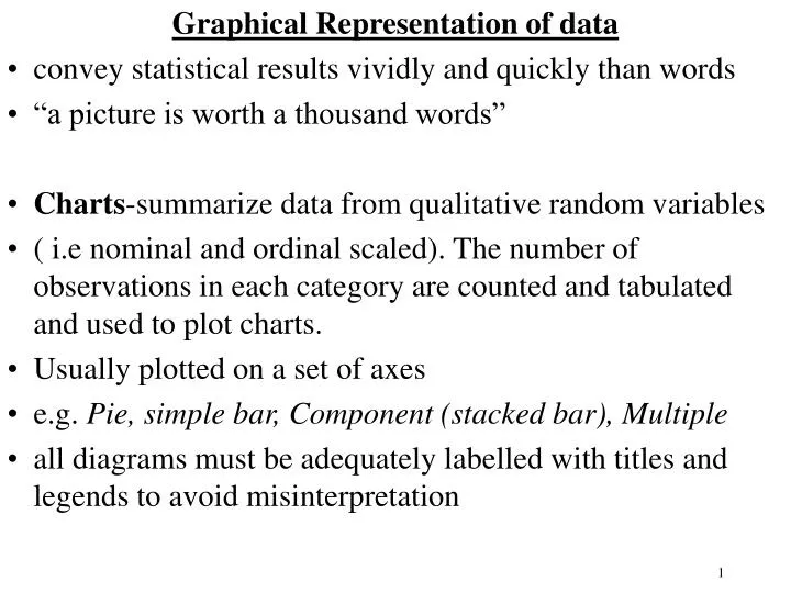
Graphical Representation of data convey statistical results vividly and quickly than words

1. Graphical Representation of data • convey statistical results vividly and quickly than words • “a picture is worth a thousand words” • Charts-summarize data from qualitative random variables • ( i.e nominal and ordinal scaled). The number of observations in each category are counted and tabulated and used to plot charts. • Usually plotted on a set of axes • e.g. Pie, simple bar, Component (stacked bar), Multiple • all diagrams must be adequately labelled with titles and legends to avoid misinterpretation

2. Simple Bar Chart • counts of observations are displayed as rectangular bars • the height of each bar is proportional to the importance or frequency of the random variable component in relation to the whole • all bars are of equal width • Disadvantage:can only display information on one variable • e.g Residential location of delegates to a conference • Northern Suburbs 156 • Southern Suburbs 234 • Avenues 144 • Countryside 66

3. Construction Notes-Simple Bar Chart • categories of the random variable are displayed on the horizontal (x-axis) • the vertical (y-axis) can be expressed in either % (relative) terms i.e showing the percentage of the respondents per residential area, or in absolute terms (i.e. the number of observations given as the frequency • the height of each bar is important. It shows the relative contribution of each category to the whole ( sum of heights =100% if using percentages) or equal to the total number of observations if using absolute terms • bars must be of equal thickness (width) to avoid distortion of category importances, but neither the order of the categories on the x axis nor the choice of bar thickness is important

5. Component Bar Chart • overcomes the limitation of a simple bar chart • allows outcomes of two or more variables to be displayed simultaneously on a single chart • each category bar of one random variable is split into sections • each section corresponds to the relative importance of each category of the second random variable • Residential Area House Flat TOTAL Northern Suburbs 102 54 156 Southern Suburbs 188 46 234 Avenues 78 66 144 CountrySide 56 10 66 TOTAL 424 176 600

6. It may be necessary to convert data to % (relative frequencies) before grouping to allow comparison between components to be made without distortion • Residential Area House Flat TOTAL Northern Suburbs 17 9 26 Southern Suburbs 31 8 39 Avenues 13 11 24 Country Side 9 2 11 TOTAL 63 37 100 • Construction Construct a simple bar chart on the first random variable( location) and then divide each bar proportionately on the second variable (dwelling type)

8. Multiple Bar Chart • more than one variable can be plotted on a single chart • variables and their categories are displayed on separate bars • categories can be compared and trends can be observed • e.g • Residential Area House Flat TOTAL Northern Suburbs 17 9 26 Southern Suburbs 31 8 39 Avenues 13 11 24 Country Side 9 2 11 TOTAL 63 37 100

10. Pie Chart • A circle divided into segments • segment size is proportional to frequency of the data category relative to the whole • expressed in % terms • best for categorical data Steps for Construction • Add all variable values under study • express each variable as a fraction of the total • multiply each fraction by 360 to set the angle in each segment • segment the circle accordingly • shade each segment differently

11. Pie Chart Africa University 1999 Graduands Faculty No. of graduands FANR 96 FMA 85 FOE 70 FOT 63 • Represent the above data on a pie chart

12. Line Graph • Displays data using lines • points are joined using straight lines • useful for showing movements in a given variable over time • also referred to as Time Series graph • more than 2 variables can be superimposed for comparisons • exercise

14. A frequency distribution is a grouping of data into categories showing the number of items falling in each category Histogram • a set of rectangular column bars used to display a frequency distribution • heights of rectangles are proportional to the frequency of each class or category • can be of same or varying width • they are drawn without leaving spaces between bars • can be an absolute or relative frequency histogram Cumulative frequency = sum of frequencies up/down to a certain threshold value

15. Histogram Construction Steps • Find midpoints of class intervals • plot the midpoints using dots • connect bars at class limits • intervals are continuous and can not be re-ordered e.g Age Range of Workshop Participants

17. Frequency Polygons • lines derived from histograms • join the midpoints of the tops of column bars using straight lines Frequency Curves • derived from frequency polygons by smoothening (removing angles) • Cumulative Frequency curve (Ogive) • A special type of frequency curve • plots of variables versus cumulative frequency • for depicting how many observations fall below or above a certain threshold value • two types (less than ogive, more than ogive)

18. Ogive Construction Steps • Create an extra class below the first class • sum all the frequencies below the current class upper limit • add the current class frequency to the immediately preceding frequencies • Office space in a set of blocks exercise plot

19. Pictograms • Picture-like or iconic symbols to display statistical data • sizes are drawn to a definite scale for comparison purposes • provide an immediate visual impact Disadvantages. -not exact e.g Number of telephone lines installed in Harare Year Number of lines (in thousands) 1991 3 1992 5 1993 7

20. No. of installed lines in Harare (000s                1991 1992 1993

21. Data Classification • The transformation of raw data into a frequency distribution • no element should be left unclassified • steps:arrange data (ascending/descending ) • determine no. of classes/categories • Determine the class interval/width (Range/C) • Assign each item to a particular class • e.g. No. of days between re-order levels for a particular range of clothing • 18 26 15 17 7 27 24 17 10 17 23 29 28 18 10 23 16 9 12 26 5 12 23 22 24 14 16 26 19 22