Download
1 / 22

E N D
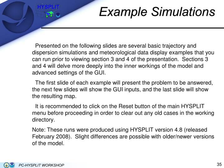
Example Simulations Presented on the following slides are several basic trajectory and dispersion simulations and meteorological data display examples that you can run prior to viewing section 3 and 4 of the presentation. Sections 3 and 4 will delve more deeply into the inner workings of the model and advanced settings of the GUI. The first slide of each example will present the problem to be answered, the next few slides will show the GUI inputs, and the last slide will show the resulting map. It is recommended to click on the Reset button of the main HYSPLIT menu before proceeding in order to clear out any old cases in the working directory. Note: These runs were produced using HYSPLIT version 4.8 (released February 2008). Slight differences are possible with older/newer versions of the model. PC-HYSPLIT WORKSHOP
Example 1: Multiple Trajectories Source Location: Dayton, Ohio (39.90N, 84.20W) @ 10 and 750 meters AGL Date/Time: December 19, 2005 @ 1800 UTC Duration: Forward 48 hours Meteorology: NAM 12 km Display: Zoom set to 80% Endpoint labels every 6 hours Vertical display coordinate set to Meters-agl Optional Google Earth PC-HYSPLIT WORKSHOP
Example 1: Inputs PC-HYSPLIT WORKSHOP
Example 1: Results PC-HYSPLIT WORKSHOP
Example 2: Back Trajectory Source Location: Nashville, TN (36.13N, 86.68W) @ 750 meters AGL Date/Time: December 22, 2005 @ 1400 UTC Duration: Backward 72 hours Meteorology: GFS Display: Zoom set to 80% Endpoint labels every 12 hours Vertical display coordinate set to Meters-agl Optional Google Earth PC-HYSPLIT WORKSHOP
Example 2: Inputs PC-HYSPLIT WORKSHOP
Example 2: Results PC-HYSPLIT WORKSHOP
Example 3: Simple Dispersion Source Location: Phoenix. AZ (33.43N, 112.02W) @ 10 meters AGL Source Duration: 1 unit/hr source emission for 2 hours Date/Time: December 20, 2005 @ 1900 UTC Duration: Forward, 12 hours Output: 12-hour average concentration between the surface and 100 meters Grid Spacing: 0.05 degrees latitude and longitude Grid Span: 20.0 degrees latitude and longitude Deposition: None Meteorology: NAM 12 km Display: Zoom set to 50% Optional Google Earth PC-HYSPLIT WORKSHOP
Example 3: Inputs PC-HYSPLIT WORKSHOP
Example 3: Inputs PC-HYSPLIT WORKSHOP
Example 3: Inputs PC-HYSPLIT WORKSHOP
Example 3: Results PC-HYSPLIT WORKSHOP
Example 4: Simple Dispersion Source Location: Phoenix. AZ (33.43N, 112.02W) @ 10 meters AGL Source Duration: 1 unit/hr source emission for 2 hours Date/Time: December 20, 2005 @ 1700 UTC Duration: Forward, 6 hours Output: 1-hour average concentration between the surface and 100 meters Grid Spacing: 0.01 degrees latitude and longitude Grid Span: 10.0 degrees latitude and longitude Deposition: None Meteorology: NAM 12 km Display: Zoom set to 100% Center plot over the source and add four 20 km rings Add county map background (file countymap) Fix exponential contours Optional: Create animated gif image PC-HYSPLIT WORKSHOP
Example 4: Inputs PC-HYSPLIT WORKSHOP
Example 4: Inputs PC-HYSPLIT WORKSHOP
Example 4: Inputs PC-HYSPLIT WORKSHOP
Example 4: Results PC-HYSPLIT WORKSHOP
Example 5: Meteorology From the last case, investigate why the plume initially moved to the NW and then to the SE using HYSPLIT’s contour and profile program. Source Location: Phoenix. AZ (33.43N, 112.02W) Date/Time: December 20, 2005 between 1500-0000 UTC Meteorology: NAM 12 km Display: Show 10 meters wind vector maps Profile output at source location from 1500-0000 UTC using the Polar coordinate system to show wind direction and speed. (This may take a few minutes to generate.) Notes: The NAMF12 dataset begins with December 19, 2005 @ 1200 UTC and has data every 3 hours, which can be determined by running profile. PC-HYSPLIT WORKSHOP
Example 5: Contour Inputs PC-HYSPLIT WORKSHOP
Example 5: Results Approximate location of source PC-HYSPLIT WORKSHOP
Example 5: Profile Inputs PC-HYSPLIT WORKSHOP
Example 5: Results • Wind Direction and Speed at 1000 hPa • Date/Time WDIR WSPD • 20/1500 114.2 1.4 • 20/1800 155.7 0.5 • 20/2100 288.2 1.5 • 21/0000 294.5 2.6 PC-HYSPLIT WORKSHOP