Download
1 / 26
260 likes | 433 Views
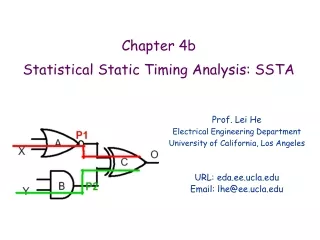
Non-Linear Statistical Static Timing Analysis for Non-Gaussian Variation Sources. Lerong Cheng, Injun Xiong, Lei He DAC 2007. Outline. Before beginning Introduction Modeling Atomic Operation Experimental Result Conclusion. Before beginning. Problem: Process variations

E N D
Non-Linear Statistical Static Timing Analysis for Non-Gaussian Variation Sources Lerong Cheng, Injun Xiong, Lei He DAC 2007
Outline • Before beginning • Introduction • Modeling • Atomic Operation • Experimental Result • Conclusion
Before beginning • Problem: Process variations • Solve: Statistical Static Timing Analysis, SSTA • The goal of SSTA is to parameterize timing characteristics of the timing graph as a function of random variables.
Before beginning • Monte Carlo method A Monte Carlo method is a computational algorithm that relies on repeated random sampling to compute its results. And it is also to be used when it is infeasible or impossible to compute an exact result with a deterministic algorithm.
Before beginning • Gaussian or Normal distribution: • PDF (probability density function) • mean • Standard Deviation
Before beginning • Triangle distribution • Uniform distribution
Before beginning • MomentGiven a random variable with probability density function , the th moment of is the value • Central moment The th moment of about the meanis the value • Raw moment The raw moments can be expressed as terms of the central moments using the inverse binomial transform
Introduction • More complicated or large-scale variation sources are taken into account in the nanometer manufacturing regime • The linear dependency of delay on the variation sources is also not accurate
Introduction • Both nonlinear delay dependency and non-Gaussian variation sources are handled simultaneously for timing analysis. • All statistical atomic operations are performed efficiently via either closed-form formulas or one-dimensional lookup tables. • The complexity of the n2SSTA algorithm is linear in both variation sources and circuit sizes.
Modeling • Let the process parameters are modeled as a random variable Xi . In general, delay function can be described as by Taylor expansion as an approximation is called the quadratic delay model. This model based on Gaussian assumption. P.S. Taylor expansion
Modeling • Because not all variation sources are Gaussian, and then is called the general canonical form.Xi: global sources of variation Xr: purely independent random variation
Modeling • Let all variation sources are centered with zero mean, i.e. Then the tth-order raw moments, i.e. is easy to compute.For example, the first three central moments of D are The mean of D is U1,The variance of D is U2,The skewness of D is U3/σ2. P.S. The nth central moment of the probability distribution of a random variable X is
Atomic Operation • To compute the arrival time, four atomic operations are sufficienti.e., addition, subtraction, maximum, minimum • Given D1 and D2 in the form then and .
Atomic Operation • Add Operation can done straight-forwardly. i.e., d0=d01+d02, ai=ai1+ai2, bi=bi1+bi2
Atomic Operation • Max Operation is the hardest operation. • compute the joint PDF of D1 and D2 • compute the raw moments of max(D1,D2) • compute the joint moments between max(D1,D2) and variation sources Xi • reconstruct the general canonical form of D=max(D1,D2)
Compute The Joint PDF • Via its first K orders of Fourier series where and where is the Fourier transformation. So we can pre-calculate all and store these results into a 1D lookup table for SSTA . P.S. Fourier series
Compute The Raw Moment • The raw moments Mt= E [max(D1,D2)t] can be computed by According to Fourier Series, Mt cam be written as where Then, raw moment can be evaluated by closed form formulas efficiently.
Compute The Joint Moment • The Joint PDF of is Then can be compute easily by 1D lookup table and closed form formulas.
General Canonical Form • To reconstruct D=max(D1,D2) into we need to determine d0, ai, bi, ar, br. • Match the joint moment of Xi and max(D1,D2) to the third-order central moments of max(D1,D2) then ai, bi can be obtained. • And d0 can be obtained by the first central moment of max(D1,D2) .
Verification • To compare with Monte Carlo simulation, it is accurate not only mean and variance, but also the skewness.
Complexity Analysis • Based on either closed-form formulas or one-dimensional lookup tables, the complexity of one max operation is O(K3N).K: the highest order for Fourier SeriesN: the number of variation source
Experimental Result • Apply to the ISCAS89 suite of benchmarks, and compared with the golden Monte Carlo simulation of 100,000 runs by using Uniform Variation Sources and Tri-angle Variation Sources, i.e., non-Gaussian and non-linear dependency.
Experimental Result • And the PDF comparison result
Experimental Result • Compare n2SSTA with linSSTA by assuming Gaussian variations and linear delay model.
Conclusion • The n2SSTA technique handle both nonlinear delay dependency and non-Gaussian variation sources using closed form formulas and one-dimensional lookup table to compute atomic operations, and it is not only accurate but also uses linear time.