Download
1 / 54
540 likes | 620 Views
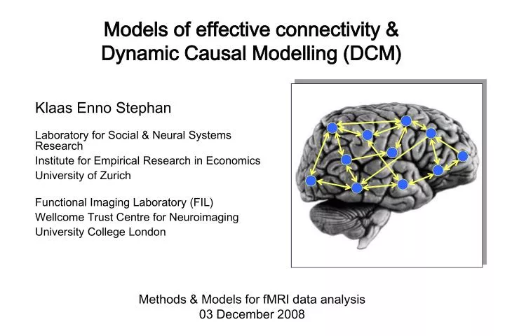
Models of effective connectivity & Dynamic Causal Modelling (DCM). Klaas Enno Stephan Laboratory for Social & Neural Systems Research Institute for Empirical Research in Economics University of Zurich Functional Imaging Laboratory (FIL) Wellcome Trust Centre for Neuroimaging

E N D
Models of effective connectivity &Dynamic Causal Modelling (DCM) Klaas Enno Stephan Laboratory for Social & Neural Systems Research Institute for Empirical Research in Economics University of Zurich Functional Imaging Laboratory (FIL) Wellcome Trust Centre for Neuroimaging University College London Methods & Models for fMRI data analysis03 December 2008
Overview • Brain connectivity: types & definitions • anatomical connectivity • functional connectivity • effective connectivity • Psycho-physiological interactions (PPI) • Dynamic causal models (DCMs) • DCM for fMRI: Neural and hemodynamic levels • Parameter estimation & inference • Applications of DCM to fMRI data • Design of experiments and models • Some empirical examples and simulations
Connectivity A central property of any system Communication systems Social networks (internet) (Canberra, Australia) FIgs. by Stephen Eick and A. Klovdahl;see http://www.nd.edu/~networks/gallery.htm
Structural, functional & effective connectivity • anatomical/structural connectivity= presence of axonal connections • functional connectivity = statistical dependencies between regional time series • effective connectivity = causal (directed) influences between neurons or neuronal populations Sporns 2007, Scholarpedia
Anatomical connectivity • neuronal communication via synaptic contacts • visualisation by tracing techniques • long-range axons “association fibres”
Diffusion-weighted imaging Parker & Alexander, 2005, Phil. Trans. B
Diffusion-weighted imaging of the cortico-spinal tract Parker, Stephan et al. 2002, NeuroImage
1. Connections are recruited in a context-dependent fashion Local functions are context-sensitive: They depend on network activity.
NMDA receptor 2. Connections show plasticity • synaptic plasticity = change in the structure and transmission properties of a chemical synapse • critical for learning • can occur both rapidly and slowly • NMDA receptors play a critical role • NMDA receptors are regulated by modulatory neurotransmitters like dopamine, serotonine, acetylcholine Gu 2002, Neuroscience
Different approaches to analysing functional connectivity • Seed voxel correlation analysis • Eigen-decomposition (PCA, SVD) • Independent component analysis (ICA) • any other technique describing statistical dependencies amongst regional time series
Seed-voxel correlation analyses • Very simple idea: • hypothesis-driven choice of a seed voxel → extract reference time series • voxel-wise correlation with time series from all other voxels in the brain seed voxel
Drug-induced changes in functional connectivity Finger-tapping task in first-episode schizophrenic patients: voxels that showed changes in functional connectivity (p<0.005) with the left ant. cerebellum after medication with olanzapine Stephan et al. 2001, Psychol. Med.
Does functional connectivity not simply correspond to co-activation in SPMs? regional response A1 regional response A2 task T No, it does not - see the fictitious example on the right: Here both areas A1 and A2 are correlated identically to task T, yet they have zero correlation among themselves: r(A1,T) = r(A2,T) = 0.71 but r(A1,A2) = 0 ! Stephan 2004, J. Anat.
Pros & Cons of functional connectivity analyses • Pros: • useful when we have no experimental control over the system of interest and no model of what caused the data (e.g. sleep, hallucinatons, etc.) • Cons: • interpretation of resulting patterns is difficult / arbitrary • no mechanistic insight into the neural system of interest • usually suboptimal for situations where we have a priori knowledge and experimental control about the system of interest models of effective connectivity necessary
For understanding brain function mechanistically, we need models of effective connectivity, i.e.models of causal interactions among neuronal populations.
Some models for computing effective connectivity from fMRI data • Structural Equation Modelling (SEM) McIntosh et al. 1991, 1994; Büchel & Friston 1997; Bullmore et al. 2000 • regression models (e.g. psycho-physiological interactions, PPIs)Friston et al. 1997 • Volterra kernels Friston & Büchel 2000 • Time series models (e.g. MAR, Granger causality)Harrison et al. 2003, Goebel et al. 2003 • Dynamic Causal Modelling (DCM)bilinear: Friston et al. 2003; nonlinear: Stephan et al. 2008
Overview • Brain connectivity: types & definitions • anatomical connectivity • functional connectivity • effective connectivity • Psycho-physiological interactions (PPI) • Dynamic causal models (DCMs) • DCM for fMRI: Neural and hemodynamic levels • Parameter estimation & inference • Applications of DCM to fMRI data • Design of experiments and models • Some empirical examples and simulations
Psycho-physiological interaction (PPI) Task factor GLM of a 2x2 factorial design: Task B Task A main effect of task TA/S1 TB/S1 Stim 1 main effect of stim. type Stimulus factor interaction Stim 2 TB/S2 TA/S2 We can replace one main effect in the GLM by the time series of an area that shows this main effect. E.g. let's replace the main effect of stimulus type by the time series of area V1: main effect of task V1 time series main effect of stim. type psycho- physiological interaction Friston et al. 1997, NeuroImage
SPM{Z} V5 activity time V1 V5 V5 attention V5 activity no attention V1 activity Attentional modulation of V1→V5 Attention = V1 x Att. Friston et al. 1997, NeuroImage Büchel & Friston 1997, Cereb. Cortex
V1 V5 V5 V1 attention attention PPI: interpretation Two possible interpretations of the PPI term: V1 V1 Modulation of V1V5 by attention Modulation of the impact of attention on V5 by V1
Two PPI variants • "Classical" PPI: • Friston et al. 1997, NeuroImage • depends on factorial design • in the GLM, physiological time series replaces one experimental factor • physio-physiological interactions: two experimental factors are replaced by physiological time series • Alternative PPI: • Macaluso et al. 2000, Science • interaction term is added to an existing GLM • can be used with any design
• • • Task-driven lateralisation Does the word contain the letter A or not? letter decisions > spatial decisions group analysis (random effects),n=16, p<0.05 corrected analysis with SPM2 time Is the red letter left or right from the midline of the word? spatial decisions > letter decisions Stephan et al. 2003, Science
Bilateral ACC activation in both tasks –but asymmetric connectivity ! group analysisrandom effects (n=15) p<0.05, corrected (SVC) IFG left ACC (-6, 16, 42) Left ACC left inf. frontal gyrus (IFG):increase during letter decisions. letter vs spatialdecisions IPS spatial vs letterdecisions right ACC (8, 16, 48) Right ACC right IPS:increase during spatial decisions. Stephan et al. 2003, Science
PPI single-subject example letterdecisions spatialdecisions bVS= -0.16 bL= -0.19 spatialdecisions letterdecisions Signal in right ant. IPS Signal in left IFG bVS=0.50 bL=0.63 Signal in right ACC Signal in left ACC Left ACC signal plotted against left IFG Right ACC signal plotted against right IPS Stephan et al. 2003, Science
Pros & Cons of PPIs • Pros: • given a single source region, we can test for its context-dependent connectivity across the entire brain • easy to implement • Cons: • very simplistic model: only allows to model contributions from a single area • ignores time-series properties of data • application to event-related data relies deconvolution procedure (Gitelman et al. 2003, NeuroImage) • operates at the level of BOLD time series sometimes very useful, but limited causal interpretability; in most cases, we need more powerful models
Overview • Brain connectivity: types & definitions • anatomical connectivity • functional connectivity • effective connectivity • Psycho-physiological interactions (PPI) • Dynamic causal models (DCMs) • DCM for fMRI: Neural and hemodynamic levels • Parameter estimation & inference • Applications of DCM to fMRI data • Design of experiments and models • Some empirical examples and simulations
LG left FG right LG right FG left Example: a linear system of dynamics in visual cortex LG = lingual gyrus FG = fusiform gyrus Visual input in the - left (LVF) - right (RVF)visual field. x4 x3 x1 x2 RVF LVF u2 u1
LG left FG right LG right FG left Example: a linear system of dynamics in visual cortex LG = lingual gyrus FG = fusiform gyrus Visual input in the - left (LVF) - right (RVF)visual field. x4 x3 x1 x2 RVF LVF u2 u1 systemstate input parameters state changes effective connectivity externalinputs
LG left FG right LG right FG left Extension: bilinear dynamic system x4 x3 x1 x2 CONTEXT RVF LVF u2 u3 u1
Dynamic Causal Modelling (DCM) Hemodynamicforward model:neural activityBOLD Electromagnetic forward model:neural activityEEGMEG LFP Neural state equation: fMRI EEG/MEG simple neuronal model complicated forward model complicated neuronal model simple forward model Stephan & Friston 2007, Handbook of Brain Connectivity inputs
x λ y Basic idea of DCM for fMRI(Friston et al. 2003, NeuroImage) • Using a bilinear state equation, a cognitive system is modelled at its underlying neuronal level (which is not directly accessible for fMRI). • The modelled neuronal dynamics (x) is transformed into area-specific BOLD signals (y) by a hemodynamic forward model (λ). The aim of DCM is to estimate parameters at the neuronal level such that the modelled BOLD signals are maximally similar to the experimentally measured BOLD signals.
Neural state equation intrinsic connectivity modulation of connectivity direct inputs modulatory input u2(t) driving input u1(t) t t y BOLD y y y λ hemodynamic model activity x2(t) activity x3(t) activity x1(t) x neuronal states integration Stephan & Friston (2007),Handbook of Brain Connectivity
Bilinear DCM driving input modulation Two-dimensional Taylor series (around x0=0, u0=0): Bilinear state equation:
u 1 u 2 Z 1 Z 2 Example: context-dependent decay u1 stimuli u1 context u2 u2 - + - x1 x1 + x2 + x2 - - Penny, Stephan, Mechelli, Friston NeuroImage (2004)
DCM parameters = rate constants Integration of a first-order linear differential equation gives anexponential function: The coupling parameter a thus describes the speed ofthe exponential change in x(t) Coupling parameter a is inverselyproportional to the half life of z(t):
t The hemodynamic model in DCM u stimulus functions neural state equation • 6 hemodynamic parameters: important for model fitting, but of no interest for statistical inference hemodynamic state equations Balloon model • Computed separately for each area (like the neural parameters) region-specific HRFs! BOLD signal change equation Friston et al. 2000, NeuroImage Stephan et al. 2007, NeuroImage
u stimulus functions neural state equation t hemodynamic state equations Balloon model BOLD signal change equation The hemodynamic model in DCM Stephan et al. 2007, NeuroImage
How interdependent are our neural and hemodynamic parameter estimates? A B C h ε r,A r,B r,C Stephan et al. 2007, NeuroImage
Bayesian statistics new data prior knowledge posterior likelihood ∙ prior Bayes theorem allows one to formally incorporate prior knowledge into computing statistical probabilities. In DCM: empirical, principled & shrinkage priors. The “posterior” probability of the parameters given the data is an optimal combination of prior knowledge and new data, weighted by their relative precision.
Shrinkage priors Small & variable effect Large & variable effect Small but clear effect Large & clear effect
ηθ|y stimulus function u Overview:parameter estimation neural state equation • Combining the neural and hemodynamic states gives the complete forward model. • An observation model includes measurement errore and confounds X (e.g. drift). • Bayesian parameter estimationby means of a Levenberg-Marquardt gradient ascent, embedded into an EM algorithm. • Result:Gaussian a posteriori parameter distributions, characterised by mean ηθ|y and covariance Cθ|y. parameters hidden states state equation observation model modelled BOLD response
Inference about DCM parameters:Bayesian single-subject analysis • Gaussian assumptions about the posterior distributions of the parameters • Use of the cumulative normal distribution to test the probability that a certain parameter (or contrast of parameters cT ηθ|y) is above a chosen threshold γ: • By default, γ is chosen as zero ("does the effect exist?"). ηθ|y
LG left FG right LG right FG left Bayesian single subject inference LD|LVF p(cT>0|y) = 98.7% 0.34 0.14 0.13 0.19 LD LD 0.44 0.14 0.29 0.14 0.01 0.17 -0.08 0.16 LD|RVF RVF stim. LVF stim. Contrast:Modulation LG right LG links by LD|LVF vs. modulation LG left LG right by LD|RVF Stephan et al. 2005, Ann. N.Y. Acad. Sci.
Inference about DCM parameters: Bayesian fixed-effects group analysis Under Gaussian assumptions this is easy to compute: Because the likelihood distributions from different subjects are independent, one can combine their posterior densities by using the posterior of one subject as the prior for the next: group posterior covariance individual posterior covariances group posterior mean individual posterior covariances and means
Inference about DCM parameters:group analysis (classical) • In analogy to “random effects” analyses in SPM, 2nd level analyses can be applied to DCM parameters: Separate fitting of identical models for each subject Selection of bilinear parameters of interest one-sample t-test:parameter > 0 ? paired t-test:parameter 1 > parameter 2 ? rmANOVA:e.g. in case of multiple sessions per subject
Overview • Brain connectivity: types & definitions • anatomical connectivity • functional connectivity • effective connectivity • Psycho-physiological interactions (PPI) • Dynamic causal models (DCMs) • DCM for fMRI: Neural and hemodynamic levels • Parameter estimation & inference • Applications of DCM to fMRI data • Design of experiments and models • Some empirical examples and simulations
Any design that is good for a GLM of fMRI data. What type of design is good for DCM?
GLM vs. DCM DCM tries to model the same phenomena as a GLM, just in a different way: It is a model, based on connectivity and its modulation, for explaining experimentally controlled variance in local responses. No activation detected by a GLM → inclusion of this region in a DCM is useless! Stephan 2004, J. Anat.
Task factor Stim1/ Task A Stim2/Task A Task B Task A TA/S1 TB/S1 Stim 1 GLM X1 X2 Stimulus factor Stim 2 TB/S2 TA/S2 Stim 1/ Task B Stim 2/ Task B Stim1 DCM X1 X2 Stim2 Task A Task B Multifactorial design: explaining interactions with DCM Let’s assume that an SPM analysis shows a main effect of stimulus in X1 and a stimulus task interaction in X2. How do we model this using DCM?