Download
1 / 46
480 likes | 689 Views
Modelling global Tropospheric Ozone: Implications for Future Air Quality and Climate. David Stevenson Institute for Meteorology University of Edinburgh Thanks to: Colin Johnson, Dick Derwent, Bill Collins (Met. Office). Talk Structure. Some background about tropospheric ozone

E N D
Modelling global Tropospheric Ozone: Implications for Future Air Quality and Climate David Stevenson Institute for Meteorology University of Edinburgh Thanks to: Colin Johnson, Dick Derwent, Bill Collins (Met. Office)
Talk Structure • Some background about tropospheric ozone • Describe the chemistry-climate model • Model comparisons with observations • Model predictions • The future
Tropospheric Ozone (O3) • Air Pollutant • City and regional-scale photochemical smogs • Damage to Vegetation • Human health – attacks tissue • Greenhouse gas • Third most potent after CO2 and CH4 • Strong spatial variation in forcing
Human health effects of ozone Damaged lung Healthy lung It makes you cry
Observed Ozone trends European mountain sites
1970-1997 ozone sonde data NH mid-latitude free troposphere IPCC, 2001
Radiative forcing 1750-2000 (IPCC, 2001) CO2 1.5 W m-2 CH4 0.5 W m-2 Trop O3 0.35 W m-2
Trop. Ozone radiative forcing1750-2000 W m-2 This is a model result IPCC, 2001
IPCC models DO3 2000-2100 Large range, particularly in tropical UT
STOCHEM • Lagrangian chemistry-transport model • 50,000 air parcels • Coupled 3 hourly to HadAM3/HadCM3 • AGCM grid: 3.75° x 2.5° x 58/19 levels • CTM output: 5° x 5° x 22 levels • 70 chemical species • CH4-CO-NOx-Hydrocarbons • Isoprene, PAN, Acetone, CH3CHO, etc. • 5-minute chemical timestep
Air parcel centres Eulerian grid from GCM provides meteorology Interpolate met. data for each air parcel STOCHEM Global Chemistry Model Framework
For each air parcel • Advection • 4th order Runge-Kutta Dt=1 hr • Plus small random component (=diffusion) • Emission & deposition fluxes • Integrate chemistry • Photochemistry • Gas phase chemistry • Aqueous phase chemistry • Mixing • with surrounding parcels • convective mixing • boundary layer mixing
Stratospheric O3 OH O3 + hn → O(3P) + O2 O3 + hn → O(1D) + O2 NO2 NO ‘Odd oxygen’ O(1D) + M → O(3P) HO2 O(3P) + O2 + M → O3 O(1D) O(3P) NOy losses O3 losses CO CH4 VOC Dry deposition Anthropogenic & Natural emissions O3 + NO → NO2 + O2 O3 NO2 + hn → O(3P) + NO
Use STOCHEM to look at some of the important factors for future European O3 • European emissions • Northern hemisphere emissions • Mix & location of emissions • Rising levels of methane • Climate change • Changing stratospheric ozone • Land use change / changing ‘natural’ emissions
Modelling approach • Repeat experiments changing only emissions • 1990 (base year) • 2030 variants • Experiments changing both emissions and climate • First, comparison with some observations for the 1990s
Global total: 24 Tg(N) Anthropogenic NOx emissions 1990 (NB excluding biomass burning)
GOME NO2: March 1997 NO2 Column Density March 1997 (1015 molecules per cm2) P. Veefkind, KNMI
EMEP O3 monitoring sites AOT40 (ppbh) April– September 1999 (daylight hours). EMEP/TOR-2 data from NILU (A-G Hjellbrekke & S Solberg)
Model – observation comparison Surface ozone Switzerland Good agreement at a rural site Poor at a nearby urban site
Model – observation comparison Surface ozone Scandinavia Good agreement at 60°N Poor in the Arctic
Observed July daytime mean O3 1990-99 STOCHEM 1800h July mean O3
Modelling approach • Repeat experiments changing only emissions • 1990 (base year) • 2030 (IPCC SRES A2 scenario) • 2030, 1990 Europe • 2030, 1990 N. America • 2030, 1990 Asia • CH4 in 1990: 1745 ppbv (used for all above) • Further 2030 run with CH4 at 2080 ppbv • Biomass burning & natural emissions fixed
+0.3 +2.4 +14.3 Global increase: +30.1 Tg(N) Change in Anthropogenic NOx emissions 1990 to 2030 Rest of World +13.1 Based on IPCC SRES A2 scenario IPCC SRES A2 scenario
Changes in other emissions 1990 to 2030 NOx in Tg(N) CO in Tg(CO) NMVOC in Tg(C)
Surface Ozone changes 1990 to 2030 (no CH4 increase) European spring/summer 0 ppbv in North up to +8 in S JAN APR JUL OCT
Surface DO3 1990 to 2030 – component due to European emissions European emissions cause-3 to +6 ppbv JAN APR JUL OCT
Surface Ozone changes 1990 to 2030 – N. American component N. American emissions cause0 to +2 ppbv JAN APR JUL OCT
Surface Ozone changes 1990 to 2030 – Asian component Vertical section 40-45°N Asian emissions cause0 to +2 ppbv JAN APR JUL OCT
Extra O3 due to regional emissions changes Europe N.America Asia
Surface Ozone changes 1990 to 2030 (including CH4 increase) European spring/summer ~ +10 ppbv JAN APR JUL OCT
Surface Ozone changes 1990 to 2030 (excluding CH4 increase) JAN APR JUL OCT
Climate change effects • Two mammoth 110-yr coupled chemistry-climate runs (1990-2100) • Control climate; SRES A2 emissions • SRES A2 climate forcing & emissions • Johnson et al. (2001 , GRL)
SRES A2 climate SRES A2 climate SRES A2 climate Control climate Control climate Control climate Climate Change effects Surface Temperature +3.5K +3.5 K Methane / ppbv CH4 lifetime Johnson et al. 2001 GRL
SRES A2 climate Control climate N. Mid-latitude surface O3 / ppbv Large negative feedback due to increases in water vapour and O3 destruction Johnson et al. 2001 GRL
Ozone chemical production (July) 200 hPa Surface
Ozone chemical loss (July) 200 hPa Surface
O3 net chemical production (July) 200 hPa Surface
Ozone lifetime (July) 200 hPa Surface Days 5 10 20 50 100
Conclusions & remaining questions • UK spring/summer surface O3 up 6 to 10 ppbv by 2030 • European emissions: -2 to -4 ppbv • UK appears to benefit from emissions reductions in E. Europe • N. American emissions: 0 to +2 ppbv • Asian emissions: 0 to +2 ppbv • Other N. Hem emissions counteract European reductions • Global methane increase: +8 ppbv • Methane increases appear very important – these are mainly driven by developing world emissions • Climate change may reduce surface O3 • More water vapour, more O3 destruction • What about: • Other emissions scenarios ? • Changes in stratospheric ozone ? • Changes in land-use / “natural” emissions ?
Future chemistry-climate modelling • Higher resolution / nested models • Plume processing • Boundary layer effects – surface & tropopause • Resolved cloud processes – lightning, convective mixing, aqueous chemistry, washout • More coupled processes • Biosphere • ENSO – biomass burning, oceanic emissions • Emissions from and deposition to vegetation
Stratospheric O3 OH NO2 NO HO2 O(1D) O(3P) NOy losses O3 losses CO CH4 VOC Dry deposition Anthropogenic & Natural emissions O3