Download
1 / 31
330 likes | 602 Views
Visualizing Diffusion Tensor Imaging Data with Merging Ellipsoids. Wei Chen, Zhejiang University Song Zhang, Mississippi State University Stephen Correia, Brown University David Tate, Harvard University 22 April 2009, Beijing. Background. Diffusion Tensor Imaging (DTI)

E N D
Visualizing Diffusion Tensor Imaging Data with Merging Ellipsoids Wei Chen, Zhejiang University Song Zhang, Mississippi State University Stephen Correia, Brown University David Tate, Harvard University 22 April 2009, Beijing
Background • Diffusion Tensor Imaging (DTI) • Water diffusion in biological tissues. • Indirect information about the integrity of the underlying white matter.
Diffusion Tensors Primary diffusion direction
Fractional anisotropy • Degree of anisotropy -represents the deviation from isotropic diffusion
Tensor at (155,155,30) Diffusion tensor: 10^(-3)* 0.5764 -0.3668 0.1105 -0.3668 0.8836 -0.1152 0.1105 -0.1152 0.8373 Eigenvalue= 0.0003 0.0008 0.0012 Eigenvector: 0.8375 -0.1734 0.5182 0.5432 0.3669 -0.7552 -0.0592 0.9140 0.4015 Primary diffusion direction: (0.5182 -0.7552 0.4015)
FA at (155,155,30) Diffusion tensor: 10^(-3)* 0.5764 -0.3668 0.1105 -0.3668 0.8836 -0.1152 0.1105 -0.1152 0.8373 Eigenvalue= 0.0003 0.0008 0.0012 FA = 0.5133
Tensor Displayed as Ellipsoid anisotropic isotropic Courtesy: G. Kindlmann λ1 = λ2 = λ3 λ1 > λ2 > λ3 λ1 > λ2 = λ3 Eigenvectors define alignment of axes
Glyphs • Shows entire diffusion tensor information • Topography information may be lost or difficult to interpret • Too many glyphs visual clutter; too few poor representation • Integral Curves • Show topography • Lost information because a tensor is reduced to a vector • Error accumulates over curves
Our contributions • A merging ellipsoid method for DTI visualization. • Place ellipsoids on the paths of DTI integral curves. • Merge them to get a smooth representation • Allows users to grasp both white matter topography/connectivity ANDlocal tensor information. • Also allows the removal of ellipsoids by using the same method used to cull redundant fibers.
Methods 1) Compute diffusion tensors: 2) Compute integral curves: p(0) = the initial point e1 = major vector field p(t) = generated curve
Methods 3) Sampling an integral curve, and place an elliptical function at each si: Streamball method [Hagen1995] employs spherical functions λ1 = λ2 = λ3, e1 = e2 = e3 4) Construct a metaball function: R = truncation radius, siis the center of the ith ellipitical function. a = −4:0/9:0; b = 17:0/9:0; c = −22:0/9:0.
Methods 5) Define a scalar influence field: 6) The merging ellipsoids representation denotes an isosurface extracted from a scalar influence field F(S; x)
Methods Visualizing eight diffusion tensors along an integral curve with (a) glyphs, (b) standard spherical streamballs [Hagen1995], and (c) merging ellipsoids
Parameters • The degree of merging or separation depends on three factors. • 1st: the iso-value C adjusted interactively • Shows merging or un-merging • 2nd: the truncation radius R • 3rd: the placement of the ellipsoids. • Currently, uniform sampling
Parameters Visualizing eight diffusion tensors with different iso-values: (a) 0.01, (b) 0.25, (c) 0.51, (d) 0.75, (e) 0.85, (f) 0.95. The truncation radius R is 1.0.
Parameters The results with different truncation radii: (a) 0.3, (b) 0.5, (c) 1.0. In all cases, the iso-value is 0.5.
Properties • The entire merging ellipsoid representation is smooth. • A diffusion tensor produces one elliptical surface. • When two diffusion tensors are close, their ellipsoids tend to merge smoothly. If they coincide, a larger ellipsoid is generated. • Provide iso-value parameters for users to interactively change sizes of ellipsoids. • Larger: ellipsoids merge with neighbors and provide a sense of connectivity • Smaller: provide better sense of individual tensors but has limited connectivity information
Comparison • If the three eigenvectors are set as identical, our method becomes the standard streamball approach. • If a sequence of ellipsoids are continuously distributed along an integral curve, the hyperstreamline representation is yielded. • An individual elliptical function can be extended into other superquadratic functions, yielding the glyph based DTI visualization representation.
Experiments • Scalar field pre-computed • Running time dependent on the grid resolution and number of tensors • Construction costs 15 minutes to 150 minutes with the volume dimension of 2563. • Visualization of ellipsoids done interactively • Reconstruction of isosurface takes 0.5 seconds using un-optimized software implementation.
Experiments • DTI data from adult healthy control participant (age > 55). • DTI protocol: • b = 0, 1000 mm/s2 • 12 directions • 1.5 Tesla Siemens • Experimental results performed on laptop P4 2.2 GHz CPU & 2G host memory.
Box = 34mm3 • Minimum path distance = 1.7mm • Anatomic structures and relationships between tensors sagittal axial coronal axial coronal sagittal
Box = 17mm3 • Min path distance = 3.4mm • b = streamtubes • c = ellipsoids • d = merging ellipsoids • Note greater detail in d sagittal coronal axial
Same ROI • Different iso-values • a = 0.90 • b = 0.80 • c = 0.60 • d = 0.40 • Different emphases on local diffusion tensor info vs. connectivity info
Forceps major • Box = 17mm3 • Min path distance = 3.4mm • Renderings • b = streamtubes • c = ellipsoids • d = merging ellipsoids • More isotropic tensors vs. corpus callosum • Change from high to low anisotropy on same fiber seen with merging ellipsoid method axial
Differences between tensors on a single curve. • Blue = more anisotropic • Red = more isotropic • Improves ability to identify problematic fibers or problematic sections on a curve
Evaluation • Identify regions within a fiber that has low anisotropy and thus might be problematic. • Normal anatomy (e.g., crossing fibers)? • Injured? • At risk? • Adjunct to conventional quantitative tractography methods
Evaluation • Adjunct to conventional quantitative tractography methods • Activate merging ellipsoids after tract selection to visually evaluate and select fibers with low or high anisotropy, even if length is same • Group comparison and statistical correlation with cognitive and/or behavioral measures • May reveal effects otherwise masked by larger number of normal fibers in the tract-of-interest
Conclusions • A simple method for simultaneous visualization of connectivity and local tensor information in DTI data. • Interactive adjustment to enhance information about local anisotropy. • Full spectrum from individual glyphs to continuous curves
Future Directions • Statistical tests • Cingulum bundle in vascular cognitive impairment • Association with apathy? • Circularity? • Select fibers at risk based on visual inspection and then enter into statistical models? • Intra-individual variability • Inter-individual variability • Interhemispheric differences
Acknowledgements • This work is partially supported by NSF of China (No.60873123), the Research Initiation Program at Mississippi State University.
Distance between integral curves s = The arc length of shorter curve s0, s1 = starting & end points of s dist(s) = shortest distance from location s on the shorter curve to the longer curve. Tt ensures two trajectories labeled different if they differ significantly over any portion of the arc length.