Download
1 / 33
330 likes | 443 Views
Workshop 9 Scripting and Batch Processing. Introduction to CFX. Pardad Petrodanesh.Co Lecturer: Ehsan Saadati ehsan.saadati@gmail.com www.petrodanesh.ir. 3.8 x H. 40 x H. Inlet. Outlet. 4 x H. Flow Separation. q. H. Introduction.

E N D
Workshop 9Scripting and Batch Processing Introduction to CFX PardadPetrodanesh.Co Lecturer: Ehsan Saadati ehsan.saadati@gmail.com www.petrodanesh.ir
3.8 x H 40 x H Inlet Outlet 4 x H Flow Separation q H Introduction This workshop models flow over a backwards facing step with heat transfer through the lower wall. The quantities of interest are the Skin Friction Coefficient and the Stanton Number on the lower wall. The choice of turbulence model can influence these results, so you will use session files and scripts to run three simulations, each with a different turbulence model, and then compare the results.
Overview In this workshop both the mesh and the physics definition are provided. The physics definition is contained in a CCL file that you will import into CFX-Pre to define the first simulation; you will then write a Definition file. The same Definition file will be used to run all three simulations, but additional CCL will be passed to the solver at run-time to alter the turbulence model. You will write a short script to run all three simulations, providing the necessary solver arguments for each run. Lastly you will create and edit a CFX-Post session file so that post-processing output can be created for all three simulations.
Define The First Simulation • Start CFX-Pre from the CFX Launcher (do not use Workbench for this example) and create a new simulation • The first simulation will use the k-epsilon turbulence model • Import the mesh file backstep.gtm • Select File > Import > CCL • Import the file ke.ccl The physics definition is imported. The CCL file you just imported was generated by setting up the simulation in CFX-Pre and then exporting the CCL through File > Export CCL.
Examining the Setup • 1D Interpolation Functions have been used to define Inlet velocity and turbulence profiles based on experimental data • The mesh is 1 element thick with symmetry boundaries on the X-Y planes • This simplifies the simulation to 2D • There is a boundary named HeatedWall through which a constant Heat Flux is applied • The k-epsilon turbulence model is used • The second and third simulations will use the SST and the k-omega turbulence models Now take a minute to look at the simulation setup:
Write the Solver File • Click the Write Solver File icon • Enter the filename as ke.def and click Save You can now write the Definition file for the k-epsilon simulation.
Preparing CCL Files • Open a new text file in Notepad • In CFX-Pre, right-click on Default Domain in the Outline tree, and select Edit in Command Editor • Copy and paste all the text from the Command Editor to your text file The next step is to prepare CCL files that change the turbulence model and can be passed to the solver at run-time. You can use the existing CCL as a template. One way to extract the existing CCL is through the Command Editor in CFX-Pre.
Preparing CCL Files • Delete the lines Create Other Side = Off and Interface Boundary = Off under BOUNDARY: Default Domain Default and BOUNDARY: HeatedWall • Save the text file in your working directory and name it SST.ccl
If you do not know the correct CCL syntax, you can make changes in the CFX-Pre GUI and then edit the object in the Command Editor to view the syntax. Preparing CCL Files • Edit the TURBULENCE MODEL Option and the TURBULENT WALL FUNCTIONS Option located at the bottom of the file as shown: • Save the changes to SST.ccl Now you can edit the text file in Notepad TURBULENCE MODEL: Option = SST END TURBULENT WALL FUNCTIONS: Option = Automatic END TURBULENCE MODEL: Option = k epsilon END TURBULENT WALL FUNCTIONS: Option = Scalable END
Preparing CCL Files • Edit the TURBULENCE MODEL Option as shown: • Save the file as komega.ccl Now change to the k-omega turbulence model for the third simulation: TURBULENCE MODEL: Option = SST END TURBULENT WALL FUNCTIONS: Option = Automatic END TURBULENCE MODEL: Option = k omega END TURBULENT WALL FUNCTIONS: Option = Automatic END The files provided with this workshop contain a scripts directory which has copies of komega.ccl and SST.ccl. You can use these files if necessary. It is not recommended to copy and paste from Powerpoint because the formatting on some characters does not translate well to Notepad.
Create a Solver Script • Perl scripts can be run on Windows and UNIX/Linux platforms • Perl comes built-in with your CFX installation and is integrated into CCL • Perl is used elsewhere in CFX, so learning some basic Perl will allow you to add advanced features to CCL. You will see an example of this when post-processing this workshop. The next step is to create a script that will run all the simulations in the solver. You could write the script in any scripting language that can be executed on your computer. Some options are Perl, a Windows batch script (.bat) or a UNIX shell script (.sh). In this workshop you will write a Perl script. This is a good choice because:
Create a Solver Script • Open a new text file in Notepad and save it in your working directory as runsolver.pl • Enter the following text (the file is also provided in the scripts directory with the workshop) • Save the changes to runsolver.pl #! perl -w print “Running the k-epsilon simulation\n”; system “cfx5solve -def ke.def"; print “Running the SST simulation\n”; system “cfx5solve -def ke.def –ccl SST.ccl –ini ke_001.res –name SST"; print “Running the k-omega simulation\n”; system “cfx5solve -def ke.def –ccl komega.ccl –ini ke_001.res –name komega";
Notes on the Perl Script • The first two lines provide information on how Perl should interpret the script. The details are not necessary here, but you can start all your Perl scripts with these two lines • # is the comment character • system executes the command in quotes • Each statement should finish with the ; character The following provides a brief explanation of the syntax used in the Perl script:
Notes on the Perl Script • –ccl <file>.ccl: this passes the CCL file to the solver that contains the new turbulence model settings. This CCL is processed after the CCL contained in the Definition file. In CCL, when the same parameter is defined more than once, the last CCL to be processed takes precedence • -ini <file>: uses the k-epsilon results to initialize the run • -name <name>: this sets the name of the .out and .res files output by the solver. The Perl script runs the solver three times using different arguments each time. The first time the k-epsilon simulation is run by providing the Definition file to the solver. The second and third time the following additional arguments are provided:
Running the Script • In the CFX Launcher check that the Working Directory is set to the directory containing the Definition file (ke.def), the CCL files (SST.ccl, komega.ccl) and the Perl script (runsolver.pl) • Select Tools > Command Line • Type perl runsolver.pl and press Enter Starting the Command Line from the CFX Launcher is always recommended because: The Perl script will now run the simulations and generate results files. You can track the progress of the runs by opening the Solver Manager, selecting File > Monitor Run in Progress, and selecting the appropriate “_001.dir” directory. • The current directory gets set to the CFX Launcher Working Directory • A number of CFX environment variables get set. One benefit of this is you do not need to use the full path to cfx5solve in the script
Session Files in CFX-Post • Start CFD-Post from the CFX Launcher (do not load results yet) • Select Session > New Session • Session files record all the actions you perform • Set the Name to post.cse • This creates a new session file, but nothing is recorded to the file until you begin recording • Select Session > Start Recording • Select File > Load Results • Load the results file ke_001.res Once the runs have finished you can proceed to CFX-Post
Session Files in CFX-Post • Select Session > Stop Recording • The above steps have recorded the CCL used to load a results file into CFX-Post. You will use this later to load the other files, all in batch mode • Create a Vector Plot of Velocity on Sym1 • Examine Temperature on Sym1 with a User Specified Range of 293 [ K ] to 1500 [ K ] • Note the hot pocket of temperature in the recirculation zone • Select Session > Start Recording to begin recording commands again • Select Insert > Location > Polyline, and accept the default name “Polyline 1” • Choose Boundary Intersection as the Method and in the Boundary List pick HeatedWall • For Intersect With select Sym1 and then click Apply
Create New Variables • Select Insert > Variable • Set the Name to Cf x 1000 • Enter the definition in the Expression box as:1000 * Wall Shear X / (0.5 * Density * (massFlowAve(Velocity)@In^2))then click Apply • Select Insert > Variable • Set the Name to St x 1000 • Enter the definition in the Expression box asshown, then click OK:1000 * Wall Heat Transfer Coefficient / (massFlowAve(Velocity)@In * Density * Specific Heat Capacity at Constant Pressure) Next you will create new variables for the Skin Friction Coefficient (Cf) and the Stanton Number (St). Both variables will be multiplied by 1000 to give a more sensible scale. You can then create Charts showing these variables along the Polyline you just created.
Create a Chart • Select Insert > Chart, accepting the default name “Chart 1” • Switch to the Data Series tab • Set the Name to Cf-ke • Set the Location to Polyline 1 • Toggle Custom Data Selection • Set the X Axis Variable to X • Set the Y Axis Variable to Cf x 1000 • Click Apply • Click the New button Now create Charts showing these variables along the Polyline
Create a Chart • Set the Name to St-ke • Set the Location to Polyline 1 • Toggle Custom Data Selection • Set the X Axis Variable to X • Set the Y Axis Variable to St x 1000 • Click Apply • Select the Export button (next to Apply) • Set the Name to ChartKE.csv and click Save • Select File > Close, choosing not to save the state • Select Session > Stop Recording
Saving the Session File The Session file now contains commands that: • Open a results file • Create a Polyline and Charts • Export data • Close the results file The next step is to edit the Session file to make it useful for running in batch mode. A discussion of all the commands you will enter is provided at the end of the workshop. If you encounter any problems you can look at the post.cse file provided with this workshop in the scripts directory
Editing the Session File • Open your Session file post.cse in a text editor. Insert/edit the text highlighted in bold font below. This will loop over all three sets of results. COMMAND FILE: CFX Post Version = 11.0 END !foreach $res ('ke_001.res','SST_001.res','komega_001.res') !{ ! print “Processing $res\n”; ! @temp = split('_001.res',$res); ! $type = $temp[0]; DATA READER:
Editing the Session File DATA READER: Clear All Objects = false Append Results = false Apply X Offset = false Apply Y Offset = false Apply Z Offset = false Keep Camera Position = true Load Particle Tracks = true END DATA READER: Domains to Load= END > load filename=$res
Editing the Session File • Continue to make the following changes. You will need to scroll down to find these areas. This will set the Line Name for the Charts based on the results file being processed CHART LINE:Chart Line 1 Auto Chart Line Colour = On Chart Line Colour = 1.0, 0.0, 0.0 Chart Line Filename = Chart Line Style = Automatic Chart Line Type = Regular Chart Symbol Colour = 0.0, 1.0, 0.0 Chart Symbol Style = None Chart X Variable = X Chart Y Variable = CF x 1000 Line Name = Cf-$type CHART SERIES:Series 1 Chart Line Custom Data Selection = On Chart Line Filename = Chart Series Type = Regular Chart X Variable = X Chart Y Variable = Cfx1000 Histogram Y Axis Weighting = None Location = /POLYLINE:Polyline 1 Series Name = Cf-$type
Editing the Session File CHART LINE:Chart Line 2 Auto Chart Line Colour = On Chart Line Colour = 1.0, 0.0, 0.0 Chart Line Style = Automatic Chart Line Visibility = On Chart Symbol Colour = 0.0, 1.0, 0.0 Chart Symbol Style = None Fill Area = On Fill Area Options = Automatic Is Valid = True Line Name = St-$type CHART SERIES:Series 2 Chart Line Custom Data Selection = On Chart Line Filename = Chart Series Type = Regular Chart X Variable = X Chart Y Variable = Stx1000 Histogram Y Axis Weighting = None Location = /POLYLINE:Polyline 1 Series Name = St-$type
Editing the Session File • The highest Temperature in the domain • The average Skin Friction Coefficient on the Polyline • The average Stanton Number on the Polyline • Insert the text after the END statement for the Chart, near the bottom of the file, before the start of the EXPORT object: Next you will add commands to evaluate some additional quantities of interest and print them out. This part was not done during the interactive CFX-Post session. The additional quantities of interest are: END ! $maxtemp = maxVal(“Temperature","Default Domain"); ! $aveCf = lengthAve("Cf x 1000","Polyline 1"); ! $aveSt = lengthAve("St x 1000","Polyline 1"); ! printf("For $type model, Highest Temp in domain is %.0f, average Cf is %.2f, average St is %.2f\n",$maxtemp,$aveCf,$aveSt); EXPORT:
Editing the Session File • Lastly make the following changes to set a filename for each exported csv file and close the foreach loop that was started at the beginning: • Save the file in your text editor ! $exfile = "chart".$type.".csv"; EXPORT: Export File = $exfile Export Chart Name = Chart 1 Overwrite = On END >export chart > close !}
Running the Session File • At the Command Line that was opened from the CFX Launcher type cfx5post –batch post.cse and press Enter • The output will print out which results file is being processed, and the evaluated quantities for maximum Temperature, average Skin Friction Coefficient and average Stanton Number. Three csv files containing the exported Chart data will also be written to the current directory. • The csv data files can be imported into Microsoft Excel through Data > Import External Data > Import Data. Set the data to be comma de-limited • You can create a chart with the data sets. See Excel help for details. • A sample Excel file is provided with this workshop You are now ready to run the modified Session file
Data Discussion The results show reasonable agreement with the Skin Friction and Stanton Number data. Note that the SST and k-omega model give a more accurate downstream reattachment location (where the Skin Friction Coefficient is zero). It has been found that a finer mesh will produce results closer to the experimental data. You can download the validation paper that was used as the basis for this workshop from the ANSYS Customer Portal.
Discussion of Commands • foreach $res(...) • This evaluates each object inside the brackets, assigns the current value inside the bracket to $res, and then processes all the commands inside the curly brackets {…..}. Hence, $res changes for each loop • @temp = split(....); • This creates an array called “temp” by splitting the filename into parts, separated by the pattern ‘_001.res’. • $type = $temp[0]; • We now use the first element in the “temp” array as our type name. We have now extracted the first part of the results file name (e.g. ke, SST or komega) A number of Perl commands and CFX Power Syntax commands were added to the Session file. These command are outlined here. For a more complete understanding refer to a Perl manual and ANSYS CFX-Post User’s Guide > Power Syntax in ANSYS CFX in the CFX Help Documentation.
Discussion of Commands • >load filename = $res • This is a CCL action that gets the value of $res and loads it. • Line Name = Cf-$type • We change the line name so it is appended with either ke, SST, or komega, depending on which loop we are currently in • ! $maxtemp = maxVal("Temperature","Default Domain"); • This is a power syntax function that obtains the max value of a variable at a location (in this case over the entire domain) and stores the value in a variable (in this case $maxtemp). There are many more of these functions available. See the Power Syntax documentation for details.