Download
1 / 18
180 likes | 312 Views
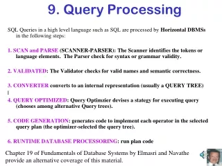
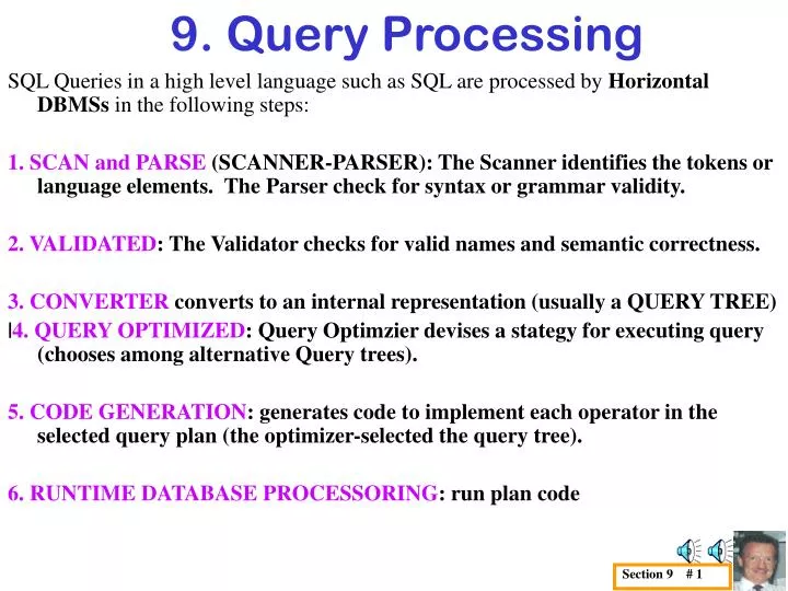
Section 9 # 1. 9. Query Processing. SQL Queries in a high level language such as SQL are processed by Horizontal DBMSs in the following steps: 1. SCAN and PARSE (SCANNER-PARSER): The Scanner identifies the tokens or language elements. The Parser check for syntax or grammar validity.

E N D
Section 9 # 1 9. Query Processing SQL Queries in a high level language such as SQL are processed by Horizontal DBMSs in the following steps: 1. SCANand PARSE (SCANNER-PARSER): The Scanner identifies the tokens or language elements. The Parser check for syntax or grammar validity. 2. VALIDATED: The Validator checks for valid names and semantic correctness. 3. CONVERTER converts to an internal representation (usually a QUERY TREE) |4. QUERY OPTIMIZED: Query Optimzier devises a stategy for executing query (chooses among alternative Query trees). 5. CODE GENERATION: generates code to implement each operator in the selected query plan (the optimizer-selected the query tree). 6. RUNTIME DATABASE PROCESSORING: run plan code
Section 9 # 2 _S______________ _C___________ _E______ |S#|SNAME |LCODE | |C#|CNAME|SITE| |S#|C#|GR| |25|CLAY |NJ5101| |8 |DSDE |ND | |32|8 |89| |32|THAISZ|NJ5102| |7 |CUS |ND | |32|7 |91| |38|GOOD |FL6321| |6 |3UA |NJ | |25|7 |68| |17|BAID |NY2091| |5 |3UA |ND .| |25|6 |76| |57|BROWN |NY2092| |32|6 |62| The CONVERTER converts to an internal representation (usually a QUERY TREE). E.g., given the database: The SQL request: SELECT S.SNAME, C.CNAME, E.GR FROM S,C,E WHERE E.GR=68 and C.SITE="ND" and S.LCODE=NJ5101 and C.C#=E.C# and S.S#=E.S#; gets SCANNED, PARSED, VALIDATED, then may get CONVERTED to query tree following the sequencing of the WHERE-clause.
Section 9 # 3 _S______________ _C___________ _E______ |S#|SNAME |LCODE | |C#|CNAME|SITE| |S#|C#|GR| |25|CLAY |NJ5101| |8 |DSDE |ND | |32|8 |89| |32|THAISZ|NJ5102| |7 |CUS |ND | |32|7 |91| |38|GOOD |FL6321| |6 |3UA |NJ | |25|7 |68| |17|BAID |NY2091| |5 |3UA |ND .| |25|6 |76| |57|BROWN |NY2092| |32|6 |62| SELECT S.SNAME, C.CNAME, E.GR FROM S,C,E WHERE E.GR=68 and C.SITE="ND" and S.LCODE=NJ5101 and C.C#=E.C# and S.S#=E.S#; M=PROJ(L)[SNAME,CNAME,GR] | L=SELECT(K.GR=68) | K=SELECT(H.SITE="ND") | H=SELECT(G.LCODE="NJ5101") | G=JOIN(F.C#=C.C#) /\ / \ JOIN(S.S#=E.S#)=F C /\ / \ S E This is simplest CONVERTER (uses the ordering in WHERE clause) CONVERTER
Section 9 # 4 M=PROJ(L)[SNAME,CNAME,GR] | | L=SELECT(K.GR=68) | | K=SELECT(H.SITE="ND") | | H=SELECT(G.LCODE="NJ5101") | | G=JOIN(F.C#=C.C#) /\ / \ JOIN(S.S#=E.S#)=F /\ / \ S E SNAME |CNAME|GR CLAY |CUS |68 S#|SNAME |LCODE |C#|GR|CNAME|SITE 25|CLAY |NJ5101|7 |68|CUS |ND S#|SNAME |LCODE |C#|GR|CNAME|SITE 25|CLAY |NJ5101|7 |68|CUS |ND CONVERTER S#|SNAME |LCODE |C#|GR|CNAME|SITE 25|CLAY |NJ5101|7 |68|CUS |ND 25|CLAY |NJ5101|6 |76|3AU |NJ S#|SNAME |LCODE |C#|GR|CNAME|SITE 25|CLAY |NJ5101|7 |68|CUS |ND 25|CLAY |NJ5101|6 |76|3AU |NJ 32|THAISZ|NJ5102|8 |89|DSDE |ND 32|THAISZ|NJ5102|7 |91|CUS |ND 32|THAISZ|NJ5102|6 |62|3UA |NJ C S#|SNAME |LCODE |C#|GR 25|CLAY |NJ5101|7 |68 25|CLAY |NJ5101|6 |76 32|THAISZ|NJ5102|8 |89 32|THAISZ|NJ5102|7 |91 32|THAISZ|NJ5102|6 |62 C#|CNAME|SITE 8 |DSDE | ND 7 |CUS | ND 6 |3UA | NJ 5 |3UA | ND S#|SNAME |LCODE 25|CLAY |NJ5101 32|THAISZ|NJ5102 38|GOOD |FL6321 17|BAID |NY2091 57|BROWN |NY2092 S#|C#|GR 32|8 |89 32|7 |91 25|7 |68 25|6 |76 32|6 |62 Let's see the results at each step.
Section 9 # 5 M=PROJ(L)[SNAME,CNAME,GR] | | G=JOIN(F.C#=K.C#) /\ / \ / \ JOIN(H.S#=L.S#)=F \ SNAME |CNAME|GR CLAY |CUS |68 Is the query tree optimal? Is this tree better? The OPTIMIZERdevises a stategy for executing the query (chooses among alternative Query trees). S#|SNAME |LCODE |C#|GR|CNAME|SITE 25|CLAY |NJ5101|7 |68|CUS |ND YES! This tree is better since the intermediate files created are much smaller!! S#|SNAME |LCODE |C#|GR 25|CLAY |NJ5101|7 |68 /\ \ / \ \ / \ \ SEL(S.LCODE=NJ5101)=H L=SEL(E.GR=68) K=SEL(C.SITE=ND) S#|SNAME |LCODE 25|CLAY |NJ5101 S#|C#|GR 25|7 |68 C#|CNAME|SITE 8 |DSDE | ND 7 |CUS | ND 5 |3UA | ND S E C S#|SNAME |LCODE 25|CLAY |NJ5101 32|THAISZ|NJ5102 38|GOOD |FL6321 17|BAID |NY2091 57|BROWN |NY2092 S#|C#|GR 32|8 |89 32|7 |91 25|7 |68 25|6 |76 32|6 |62 C#|CNAME|SITE 8 |DSDE | ND 7 |CUS | ND 6 |3UA | NJ 5 |3UA | ND
Section 9 # 6 M=PROJ(L)[SNAME,CNAME,GR] | | G=JOIN(F.C#=K.C#) /\ / \ / \ JOIN(H.S#=L.S#)=F \ SNAME |CNAME|GR CLAY |CUS |68 Note that the following could be done: • SITE attribute can be projected from K (doesn't require elimination of duplicates because it is not part of the key). • The LCODE attrib can be projected off of H (doesn't require elimination of duplicates because it is not part of the key). • S# could be projected off of F (it is part of the key but duplicate elimination could be deferred until M since it will have to be done again there anyway - thus this projection can be a "non duplicate-eliminating" projection also (which we will denote by [[ ]]). [[ ]]-projections take no time, whereas duplicate eliminating projections take a lot of time). • C# can be (non-duplicate-eliminating) projected off G (just reordering attrs and eliminating duplicates, if any). SNAME |GR|CNAME CLAY |68|CUS Even better! The intermediate files created are even smaller!! /\ \ / \ \ / \ \ H=SEL(S.LCODE=NJ5101)[[S#,SNAME]] L=SEL(E.GR=68) K=SEL(C.SITE=ND)[[C#,CNAME]] S#|SNAME |C#|GR 25|CLAY |7 |68 S#|SNAME 25|CLAY S#|C#|GR 25|7 |68 C#|CNAME 8 |DSDE 7 |CUS 5 |3UA S E S#|C#|GR 32|8 |89 32|7 |91 25|7 |68 25|6 |76 32|6 |62 C S#|SNAME |LCODE 25|CLAY |NJ5101 32|THAISZ|NJ5102 38|GOOD |FL6321 17|BAID |NY2091 57|BROWN |NY2092 C#|CNAME|SITE 8 |DSDE | ND 7 |CUS | ND 6 |3UA | NJ 5 |3UA | ND
Section 9 # 7 What have we learned about QP? GOOD RULES? a. Do SELECTS first (push to the bottom of the tree). b. Do attribute elimination part of PROJECT as soon as possible (push down). c. Only do duplicate elimination once (at top-most PROJECT only or in conjunction with a latter join step). QUERY OPTIMIZATION, then, is finding an efficient strategy to implement query requests (Automatically, Heuristically, not necessarily optimally) Note: In lower level languages, the user does the query optimization by writing the procedural code to specify all steps and order those steps. (of course there are optimizing compilers that will automatically alter your "procedures", but still you are mostly responsible for ordering). Relational queries are issued at a high level (SQL or ODBC), so that system has maximal oportunity to optimize them. HEURISTIC RULES are used to re-order query tree. (e.g., RULES a. b. c. above) . Some rules depend upon size and complexity estimates. ESTIMATION estimates the cost of different strategies and chooses the best. Challenge: Get acceptable performance (took 10 years to optimize join process acceptably so that the first viable Relational DBMSs could be successfully sold!).
Section 9 # 8 CODE GENERATION implements the operators above (e.g., SELECT, PROJECT, JOIN...) Some SELECT implementations: (Each of S2 - S6 requires a special access path.) S1. Linear search: sequentially search every record. S2. Binary search: (for selections on a clustered or ordered attribute) S3. Using indexes (or hash structures) for an equality comparison S4. Using primary index for an inequality comparison on a key (clustered). S5. Using aclustering index for "=" comparison S6. Using asecondary B+-tree index for "=", use the index set. SELECTION methods with a WHERE conjunction (AND): S7. Of the many conjunctive attributes, select 1 attribute (usually involving an "=") S8. Intersection of Rrecord Pointers: Intersect RRN-sets then retrieve records S9. If there areBitmapped Indexes, AND bitmaps CASE-1: SELECT is on an attribute with few distinct values. CASE-2: SELECT is on an attribute with uniqueness (key) or near uniqueness. S10. If there is acomposite index on the attributes involved in condition, use it. S11. If there is a composite hash function, use it. SELECTION methods when there is a WHERE disjuntion (OR): S12. If there isno access path (indexes or hash functions), use S1 (brute force). S13. If there areaccess paths, use them and UNION the results. S14. If there areBitMaps, take the OR of the bitmaps.
ENROLL ENROLL 32|89 32|91 32|91 S#|C#|GR 32|8 |89 32|7 |91 25|7 |68 25|6 |76 32|6 |62 38|6 |98 17|5 |96 RRN|S#|C#|GR 0 |17|5 |96 1 |25|7 |68 2 |25|6 |76 3 |32|8 |89 4 |32|7 |91 5 |34|6 |62 6 |38|6 |98 32|91 Section 9 # 9 Required for selections from an unordered relation with no index or access path. SELECT C#, GR FROM ENROLL WHERE S# = 32; S1. Linear search: sequentially search every record. S2. Binary search: For selections on a clustered (ordered) attribute (in this case, S#): SELECT C#, GR FROM ENROLL WHERE S# = 38; Go half way (to RRN=3), since S# < 38, go half way down what's left (to RRN= 5). Since S# < 38, go half way down what's left (to RRN= 6). Match! Output. Scan aheadand output until no match or EoF.
STUDENT STUDENT Index on S# Index always clustered on the key (here S#) for binary key search. RID|S#|SNAME | LCODE 1,0|17|BAID |NY2091 1,1|25|CLAY |NJ5101 2,0|32|THAISZ|NJ5102 2,1|38|GOOD |FL6321 3,0|57|BROWN |NY2092 RRN|S#|SNAME | LCODE 0 |25|CLAY |NJ5101 1 |32|THAISZ|NJ5102 2 |38|GOOD |FL6321 3 |17|BAID |NY2091 4 |57|BROWN |NY2092 RRN| S# 3 | 17 57| BROWN 32| THAISZ 32| THAISZ 38| GOOD 0 | 25 1 | 32 2 | 38 4 | 57 Section 9 # 10 SELECT C#, NAME FROM STUDENT WHERE S# = 32 S3. Using Indexes: (or hash structures) for an equality comparison. S4. Using primary index for an inequality comparison on a key (clustered). (Find starting point with "=", then retrieve all records beyond that point). SELECT S#,NAME FROM STUDENT WHERE S# 32 nondense Primary Index on S# RID| S# Find starting point (first S# 32) then scan ahead taking all until End 1,0| 17 2,0| 32 3,0| 57
Clustering Index on S# ENROLL=E Find first S#=32, then scan E ahead for others. RRN| S# 0 | 17 RRN|S#|C#|GR 0 |17|5 |96 1 |25|7 |68 2 |25|6 |76 3 |32|8 |89 4 |32|7 |91 5 |32|6 |62 6 |38|6 |98 32| 91 32| 62 CLAY|OUTBK 32| 89 1 | 25 3 | 32 6 | 38 S6. Using asecondary B+-tree index: For "=", use the index set (assuming a B+tree index) SELECT NAME,CITY FROM STUDENT WHERE S# = 25 *32*38* *20* n n32* n *56* n |17 20|25 32|35 38| 56|57 | 2 5|4 1|7 3| 6|0 STUDENT RRN|S#|SNAME |CITY |ST 0 |57|BROWN |NY |NY 1 |32|THAISZ|KNOB |NJ 2 |17|BAID |NY |NY 3 |38|GOOD |GATER|FL 4 |25|CLAY |OUTBK|NJ 5 |20|JOB |MRHD |MN 6 |56|BURGUM|FARGO|ND 7 |35|BOYD |FLAX |NE Section 9 # 11 SELECT C#, GR FROM ENROLL WHERE S# = 32 S5. Using a Clustered Index: for = comparison.
GOOD |GATER BURGUM|FARGO BROWN |NY S6. Using asecondary B+-tree index: For use the index set, then use sequence set (of B+) SELECT NAME,CITY FROM STUDENT WHERE S# 38 *32*38* *20* n n32* n *56* n |17 20|25 32|35 38| 56|57 | 2 5|4 1|7 3| 6|0 STUDENT RRN|S#|SNAME |CITY |ST 0 |57|BROWN |NY |NY 1 |32|THAISZ|KNOB |NJ 2 |17|BAID |NY |NY 3 |38|GOOD |GATER|FL 4 |25|CLAY |OUTBK|NJ 5 |20|JOB |MRHD |MN 6 |56|BURGUM|FARGO|ND 7 |35|BOYD |FLAX |NE Section 9 # 12
Secondary Index on ST RRN| ST 3 | FL BOYD |FLAX 5 | MN 7 | NE 6 | ND 1,4| NJ 0,2| NY *32*38* *20* n n32* n *56* n |17 20|25 32|35 38| 56|57 | 2 5|4 1|7 3| 6|0 STUDENT RRN|S#|SNAME |CITY |ST 0 |57|BROWN |NY |NY 1 |32|THAISZ|KNOB |NJ 2 |17|BAID |NY |NY 3 |38|GOOD |GATER|FL 4 |25|CLAY |OUTBK|NJ 5 |20|JOB |MRHD |MN 6 |56|BURGUM|FARGO|ND 7 |35|BOYD |FLAX |NE Section 9 # 13 SELECT NAME, CITY FROM STUDENT WHERE S#>25 and ST=NE S7. Of the many conjunctive attributes,select on1 attribute (usually 1 involving an "=") then check the other condition(s) for each retrieved record.
Secondary Index on ST RRN| ST 3 | FL BROWN |NY BURGUM|FARGO GOOD |GATER 5 | MN 7 | NE 6 | ND 1,4| NJ 0,2| NY *32*38* *20* n n32* n *56* n |17 20|25 32|35 38| 56|57 | 2 5|4 1|7 3| 6|0 STUDENT RRN|S#|SNAME |CITY |ST 0 |57|BROWN |NY |NY 1 |32|THAISZ|KNOB |NJ 2 |17|BAID |NY |NY 3 |38|GOOD |GATER|FL 4 |25|CLAY |OUTBK|NJ 5 |20|JOB |MRHD |MN 6 |56|BURGUM|FARGO|ND 7 |35|BOYD |FLAX |NE Section 9 # 14 SELECT NAME, CITY FROM STUDENT WHERE S#>38 and STNE true true true S7. Of the many conjunctive attributes,select on1 attribute (neither involve =! taking S#) then check the other condition(s) for each retrieved record.
S#-RRN-list ST-RRN-list intersection 1,7,3,6,0 0,2,7 0,7 S9. If Bitmap Indexes BMI on ST ST|bit-filter FL| 00010000 MN| 00001000 NE| 00000001 ND| 00000010 NJ| 01001000 NY| 10100000 S#|bit-filter 17| 00100000 20| 00000100 25| 00001000 32| 01000000 OR here to end (S#>25) result: 11010011 35| 00000001 OR NE, NY bitfilters: 10100001 38| 00010000 AND two for result: 10000001 56| 00000010 57| 10000000 STUDENT RRN|S#|SNAME |CITY |ST 0 |57|BROWN |NY |NY 1 |32|THAISZ|KNOB |NJ 2 |17|BAID |NY |NY 3 |38|GOOD |GATER|FL 4 |25|CLAY |OUTBK|NJ 5 |20|JOB |MRHD |MN 6 |56|BURGUM|FARGO|ND 7 |35|BOYD |FLAX |NE Section 9 # 15 S8. INTERSECTION OF RECORD POINTERS: Intersect RRN-sets then retrieve records. SELECT NAME,CITY FROM STUDENT WHERE S#>25 and (ST=NE or ST=NY); (This can be done in conjunction with any of the above methods. If the RRN-sets are stored ahead of time for particular selection criterial, then they can greatly speed up the execution. The question is, which should be generated and stored?).
Section 9 # 16 S8. INTERSECTION OF RECORD POINTERS: ANDing bitmaps, then retrieve records. SELECT NAME,CITY FROM STUDENT WHERE S#>25 and (ST=NE or ST=NY); BitMapped Indexes (BMIs) are used only for "low cardinality" attributes in DataWarehouses. (those with a small domain - ie, only a few possible values. The reason is that for low-cordinality domains (eg, MONTH, STATE, GENDER, etc.), BMI has few entries (rows) and each bitmap is quite dense (many 1-bits To see why this is so, consider two extremes. CASE-1: For a GENDER attribute in a relation with 80,000 tuples. The BMI looks like: GENDER| bit-filter Female| 0111001010100...1 Male | 1000110101011...0 Eaach bitfilter is 80,000 bits or 10KB so the index is ~20KB with only two distinct values (Note the Male entry is unnecessary since it can be calculated from Female bitfilter as the bit-compliment. Thus, the index is only ~10KB in size altogether. If a regular index were used: GENDER|RID-list Female|RID-F1, RID-F2, ..., RID-Fn Male |RID-M1, RID-M2, ..., RID-Mn Each RID takes 8 bytes (maybe more?) The size is ~640KB. Thus BMI size could be as low as ~10KB and the regular index size ~640KB.
Section 9 # 17 S8. INTERSECTION OF RECORD POINTERS: ANDing bitmaps, then retrieve records. SELECT NAME,CITY FROM STUDENT WHERE S#>25 and (ST=NE or ST=NY); BitMapped Indexes (BMIs) CASE-2: SSN attr of employee file for large company (say, with 80,000 employees) BMI: SSN |bit-filter 324-66-9870 |1000000000000...0 ... 687-99-2536 |0000000000000...1 Extant Domain (only those SSN's of existing employees) Each bitfilter 80Kb (10KB) so the index is 80,000 * ~10KB or ~800MB in size. If a regular index were used: SSN |RID 324-66-9870 |RID1 ... 687-99-2536 |RID80000 If RIDs take 8 bytes and SSN+separators take another 12 bytes,the size is ~20*80,000 bits = ~200KB Thus the BMI size could be as low as ~800,000KB and the regular index size would be ~200KB
Section 9 # 18 S10. If there is acomposite index on the attrs involved in condition, use it. If there is a composite hash function, use it Selection implementation is matter of choosing among these alternatives (possibly others?). SELECTION methods when there is a WHERE disjuntion (OR) in the condition If there is no access path (indexes or hash fctns), use S1 (brute force). If there are access paths , use them and UNION the results, or UNION the RID-sets, then get the records (rather than interesection as in the case of AND condition). If there are BitMaps, take the OR of BitMaps, then get records