Download
1 / 39
390 likes | 392 Views
Comparison of NO 2 profiles derived from MAX-DOAS measurements and model simulations. Folkard Wittrock, Katrijn Cl é mer and the NO 2 profiling team. Objectives of the Bremen workshop in November. To present the „state of the art“ in tropospheric profiling of NO 2 (and other trace gases)

E N D
Comparison of NO2 profiles derived from MAX-DOAS measurements and model simulations Folkard Wittrock, Katrijn Clémerand the NO2 profiling team EOS-AURA Science Team Meeting14-17 September 2009, Leiden
Objectives of the Bremen workshop in November • To present the „state of the art“ in tropospheric profiling of NO2 (and other trace gases) • To identify advantages but also limitations of the different methods • To collect ideas how to improve the methods and how to move on in the future e.g. harmonize MAXDOAS instruments and retrievals
MAXDOAS vs. in situ BIRA MAXDOAS VMR surface layer compared to EMPA in situ courtesy: Katrijn Clémer, BIRA
MAXDOAS vs. in situ VMR surface layer compared to Bremen in situ In situ BREAM GL
NO2 Profile Comparison 25 June 23 June • first comparisons sometimes o.k., sometimes not • challenge is to identify what causes the differences-> model study
Simulation study • IASB-BIRA has provided modeled NO2 slant columns for UV and visible, using • 8 different NO2 scenarios (profiles) • 2 aerosol loadings (AOD 0.14 and 0.54 for 477 nm) • aerosol information based on CIMEL data from Cabauw • HG phasefunction with asymmetry factor of 0.67 • Simulations for June 24, 2009 in Cabauw • 10 Elevation Angles (1,2,4,5,6,8,10,15,30,89) • SCD error based on real DOAS fit errors plus Gaussian noise • Calculations with LIDORT
Simulation study Fixed settingsfor OE retrievalalgorithms • 0 to 4 km • Apriori 1 ppb atthesurface, 0.01 ppb atthe top • Sa 100% • 2 retrievals per situationandwavelength • Height grid 50 and 200m -> In total 64 retrievals • In total 5 groups (BIRA, MPI, NIWA, iup Bremen, WSU) havecalculateddata (4 OE, one „simple“ least squaresmethod, onlyoneresultforeachsituation)
Simulation study Bremen retrieval of block profile for low aerosol (UV)
Simulation study Bremen retrieval of block profile for high aerosol (UV)
Simulation study Exponential low pollution, low aerosol
Simulation study Exponential high pollution, low aerosol
Simulation study Block low pollution, low aerosol
Simulation study Block high pollution, low aerosol
Simulation study Very shallow layer, low aerosol
Simulation study Less shallow layer, low aerosol
Simulation study Uplifted layer, low pollution, low aerosol
Simulation study Uplifted layer, high pollution, low aerosol
Simulation study Exponential low pollution, high aerosol
Simulation study Exponential high pollution, high aerosol
Simulation study Block low pollution, high aerosol
Simulation study Block high pollution, high aerosol
Simulation study Very shallow layer, high aerosol
Simulation study Less shallow layer, high aerosol
Simulation study Uplifted layer, low pollution, high aerosol
Simulation study Uplifted layer, high pollution, high aerosol
Conclusions • OE retrieval methods agree quite well to each other,… but not always to „reality“ • VC usually captured well also for difficult conditions • Viewing directions towards sun and for high SZA difficult to retrieve • Best settings for OE still open: • Finer grid gives more details, but tends to more oscillations -> Elena has the solution? • UV retrieval seems to be more stable • Is OE the best method for MAXDOAS retrievals?
Outlook • Waiting formoregroupstocontribute (e.g. JAMSTEC on simulateddata, MPI on real data), same deadlineasforaerosols -> Mid April Profiling paper: • NO2profileintercomparisonfocusing on MAXDOAS capabilitiesandusing LIDAR and in situ ascomplementarydatasets (CWG: F. Wittrock, K. Clemer, H. Irie, S. Beirle?)Drafttobewritten in April 2010 before EGU
Empa sees ca. 10 % more NO2 In situ instruments Comparison of Bremen in situ Instrument with Empa and RIVM (at ground level) Bremen - EMPA Slope : 1.11 Correlation : 0.993 Bremen – RIVM Slope : 0.985 Correlation : 0.992 • BLC instruments agree quite well
In situ instruments • deviation between surface in-situ and 200 m in-situ gives information on boundary layer mixing
In situ instruments • NO2 often not well mixed even in the lowest 200 m