Download
1 / 21
220 likes | 396 Views
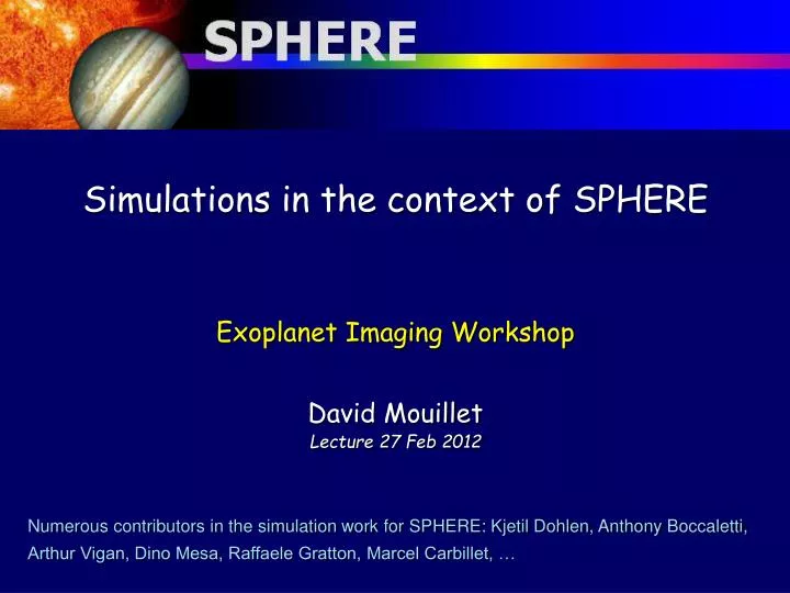
Simulations in the context of SPHERE Exoplanet Imaging Workshop David Mouillet Lecture 27 Feb 2012. Numerous contributors in the simulation work for SPHERE: Kjetil Dohlen, Anthony Boccaletti, Arthur Vigan, Dino Mesa, Raffaele Gratton, Marcel Carbillet, …. SPHERE overall presentation.

E N D
Simulations in the context of SPHERE Exoplanet Imaging Workshop David Mouillet Lecture 27 Feb 2012 Numerous contributors in the simulation work for SPHERE: Kjetil Dohlen, Anthony Boccaletti, Arthur Vigan, Dino Mesa, Raffaele Gratton, Marcel Carbillet, …
SPHERE overall presentation • Many similarities wrt GPI (see Lisa’s presentation) in terms of high level purposes, main components and challenges : • High order AO, coronagraphs, multi-wavelength differential imaging, angular differential imaging, budget analysis up to 8-10 target magnitude, … • With some significant differences: • Focus: Nasmyth vs Cassegrain (flexures, telescope vs instrument WFE) • Wavelength coverage: • A VISIBLE imager with differential polarimetry: ZIMPOL. 500-900 nm • Wider NIR simultaneous coverage: 0.95 – 1.65 mic (IFS + diff imager IRDIS, or IFS only) • Variable / Differential WFE: • pupil de-rotator, 2 ADCs: some rotating surfaces (eventhough in a predictible manner) • No « CAL » system (NIR tilt/defocus sensor only)
High frequency AO correction (41x41 act.) High stability : image / pupil control Visible – NIR Refraction correction FoV = 12.5’’ 40x40 SH-WFS in visible 1.2 KHz, RON < 1e- Beam control (DM, TT, PTT, derotation) Pola control Calibration Coronagraphic imaging: Dual polarimetry, direct BB + NB. λ = 0.5 – 0.9 µm, λ/2D @ 0.6 µm, FoV = 3.5” 0.95 – 1.35/1.65 µm λ/2D @ 0.95 µm, Spectral resolution: R = 54 / 33 FoV = 1.77” Pupil apodisation, Focal masks: Lyot, A4Q, ALC. IR-TT sensor for fine entering 0.95 – 2.32 µm; λ/2D @ 0.95 µm Differential imaging: 2 wavelengths, R~30, FoV = 12.5’’ Long Slit spectro: R~50 & 400 Differential polarization Nasmyth platform, static bench, Temperature control, cleanliness control Active vibration control Concept overview
Implementation CPI Focus 1 HWP2 De-rotator ITTM HWP1 PTTM Polar Cal Focus 2 DM Focus 4 NIR ADC VIS ADC DTTS VIS corono Focus 3 ZIMPOL WFS NIR corono DTTP IFS IRDIS
SPHERE in test environment IRDIS IFS ZIMPOL CPI (structure, damping system..) Calibration sources
Simulations: risks and difficulties • Variety of effects to be taken into account, various timescales • Needed accuracy • Metric to consider ? • Impact on final contrast performance after data reduction • Inter-dependency of various contributors to the budget • Risk: forget an important limitation source, system imperfection • Risk: in the limit of very bright targets, including only well understood defects (also considered in data reduction): syndroma of infinite performance
Simulation approach • separate limitation types: • « noise » contributors derived from mean image properties and system properties: stellar halo, detector, background, FF • speckle calibration residuals
Requirements for simulation Tools • To estimate mean image profilein various conditions (AO correction conditions, coronagraphs, filters) photon noise, FF noise… • To estimate sensitivity to WFE dependencies, in particular as a function of wavelength (various sources of chromatism), and time system specifications • to estimate long-term speckle pattern evolution • Detailed AO loop simulation system specification on stability, noise propagation, control laws, vibration filtering, impact of calib errors • IFS internal behaviour system specifications on cross-talk, samplings, detector calibration accuracy…
Baseline diffraction code • Baseline including: • Fraunhofer propagation through pupil and focal planes • AO-filtered turbulence residuals, based on analytical model: simulation of n independent realization of residuals • realistic optics wfe in terms of rms and DSP • various coronagraph types • WFE: clear distinction between before/after coronagraph, time variable, chromaticity • Limitations or effects treated on a case-by-case basis • no out-of-pupil WFE in baseline. Fresnel effects only roughly estimated for some of the most sensitive surfaces (PROPER code, see J. Krist’s presentation) • Amplitude defects: few test cases but not treated exhaustively • Chromatism not treated exhaustively: mainly residual tilt, defocus, diff WFE for IRDIS dual band imaging • Difficulty to handle very different timescales from ms to hr
Fulfilling the Requirements • To estimate mean image profilein various conditions (AO correction conditions, coronagraphs, filters) photon noise, FF noise… • To estimate sensitivity to WFE dependencies, in particular as a function of wavelength (various sources of chromatism), and time system specifications • to estimate long-term speckle pattern evolution • Detailed AO loop simulation system specification on stability, noise propagation, control laws, vibration filtering, impact of calib errors • IFS internal behaviour system specifications on cross-talk, samplings, detector calibration accuracy…
Fulfilling the Requirements IFS internal behaviour • From x,y,l cubes to simulated detector images: • Including fraction on lenslets and downstream optics • Possible detector and calibration defects • Time consuming: can often be restricted to a small part of the image • On operational point of view: definite support to data reduction testing • On Signal/performance point of view: • Some tests about sensitivity to cross-talk • Analysis not so easy ; some coupling with image spatial structure, data extraction algo, and final impact depends also on the temporal structure (in case of artifact, how wold they smooth down ?) • A point to be precised in very good performance regime (other aspects well handled) and/or if problem in terms of IFS internal calibration and signal extraction
Fulfilling the Requirements AO loop detailed study • End-2-end simulation from incoming turbulent WFE, through AO signal at each iteration and AO residual estimates • Time consuming: • Used for AO loop system analysis and specifications • Used to validate simpler analytical tools (based on DSP filtering) • NOT used for numerous overall instrument image estimates • Good feedback from tests: • good agreement between end-2-end simus and actual loop behaviour. • Validation of analytical tool • Pending confirmation concerning lowest flux
Fulfilling the Requirements Mean Images • Simple use of diffraction code, low sensitivity to exact WFE values. Main dependencies: • AO correction quality • Coronagraph • Mean wavelength. (+ also, spectral width if speckle constrast is concerned) • combined use with analytical formulae for extrapolation to numerous astrophysical cases (star type, distance, magnitude, total integraton time, individual detector integration time…) and comparison of various noise sources
Fulfilling the Requirements Sensitivity to WFE dependencies • Strong support to system specifications, with numerous and coupled system parameters, also depending on signal extraction: need for an underlying very schematic approach for differential imaging: whatever the exact signal extraction algo, we want to minimize • The chromaticity of speckle pattern obtained simultaneously • The image variability over time, with specific attention to two timescales: • Minutes : time for companion differential imaging with field rotation (or polarimetric/filter switches) • Hour: typical type for deep integration, potential re-calibration of the system • Numerous tests made with just simple differences between two distinct images: • Not representative to final perf • But good estimate to pvarious parameter sensitivity • Use of baseline diffraction code, in various conditions; Note: AO residuals not critical here.
Fulfilling the Requirements Long-term speckle pattern evolution • Support and typical example for various ADI data reduction: 4 hr continuous observation, crossing meridian, sampled with 144 mean images (1 every 100 s). • Use of diffraction code including various timescales and variability effects: • Approximative representation of turbulence residuals (not sampling AO loop iterations): average of 100 independent realization, statistics not fully converged but correlated on successive images. • Predictible WFE evolution: rotating surfaces, ADC residuals associated to airmass • Slow random effects: • Turbulence non-stationarity: seeing, windspeed • Thermal drifts effects on centering, defocus • Production of x,y,l,t cubes (limited to small number of wavelengths up to now…)
Fulfilling the Requirements Long-term speckle pattern evolution • eg: DEC = -45° from Paranal, HA = -2 -> +2 hr Airmass and Field rotation rate Evolution of pre-coro WFE var Evolution of pre-corovariabilitybetween successive images PSD of differencebetween WFE: 0 -1 PSD of differencebetween WFE: 0 -71
Fulfilling the Requirements Long-term speckle pattern evolution • eg: DEC = -45° from Paranal, HA = -2 -> +2 hr turbulence Variable de-centering r0 Wind speed
Fulfilling the Requirements Long-term speckle pattern evolution
Lessons learnt • We have the ability to simulate many effects eventhough some care/effort may be involved, and possibly some simplifying tricks (for computation time saving) • Eg from very short ot long timescales • Fresnel effects on numerous surfaces • Detailed effects internal to IFS… • A major challenge for system/performance analysis = the number of parameters involved and combination to signal extraction approach • Strong relation to system/signal: an a priori analysis of defects is needed first qualitatively => simulations provide the quantitative answer • Single parameter sensitivity analysis in context of a given system paradigm = more robust than multi-parameter investigation • Conclusions for a given system may not be extrapolated to another system • Major risk for performance prediction = missing significant contributor ??
Risk items • riskprobablyreasonable up to contrast 10 6-7 • timescalesaround minutes atvery fine levels (eventhough the system isspecified for this) • vibrations, turbulence non-stationarity • rotating surfaces, + ADC correction • thermal drifts, slow loopsresiduals • ultimate performance for WFE calibration ? (currentassumptions for simus=quite conservative): margin for improvement and upgrades • Amplitude/Fresnel/chromaticeffects, crosstalkeffects for contrasts >~10 7 • Fine detector calibration residuals ? • + the unexpected !