Download
1 / 1

E N D
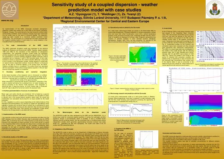
www.rec.org Introductionhe implementation of the NIRE mesoscale circulation atmospheric dispersion model was carried out in year 2000 at the Eotvos University, Budapest, Hungary. The model dynamics has been tested for artificial initial and boundary conditions. Some necessary changes have been introduced into the model code for the sake of numerical stability. The dispersion model has been coupled to a numerical weather prediction model (NCEP/ETA). The concentration of a contaminant has been calculated with the coupled modeling system. A case study for a recent situation in the Carpathian Basin is presented below. Sensitivity study of a coupled dispersion - weatherprediction model with case studiesA.Z. 1Gyongyosi (1), T. 1Weidinger (1), Zs. 2Ivanyi (2)1Department ofMeteorology, Eötvös Loránd University, 1117 Budapest Pázmány P. s. 1/A,2Regional Environmental Center for Central and Eastern Europe 2.2 Operational products yielded by the Eta model On a daily basis meteorological fields are posted on the World Wide Web for meteorological application. Predicted distribution of surface temperature, surface wind and mass field, Lifted Condensation Level (LCL), vertical temperature gradient of the convective boundary layer, integrated sensible heat flux and K-index of instability are displayed on forecast maps. Diagrams representing time variation of selected variables in some selected locations (Budapest, Nyíregyháza, Szeged, Győr, Pécs, are also presented. An example for the above mentioned fields and diagrams are given on Fig. 4and 5 below. 4. A case study At the 2 February 2006 a cold surface inversion layer was present in the Carpathian Basin (inversion case). This cold inversion was broken up by a severe cold front, and after the passing of the cold front, neutral conditions were present in the PBL with an unstable surface layer in the daytime (convection case). Temperature and dew point soundings at 12Z on the 2 February and the 6 February are plotted on Fig. 8. Temperature profiles for the inversion and convection cases were evaluated and they showed good agreement with rawinsonde measurements. The effect of a single large stack was investigated in the middle of the model domain with the following emission data: 200 m high elevated point source. Intensity: 280 m3/s @ 3000C total emission of 1000 t/day CO2. Typical CO2 profiles in the vicinity of the source in inversion and convection condition are plotted on Fig. 9, respectively. In case of inversion we got extremely high concentration near surface even in the daytime while in case of convection in the daytime we got much cleaner air. These results are in a good agreement with what we would expect. 1. The main characteristics of the NIRE modelThe NIRE mesoscale circulation model was developed at the National Institute for Resource and Environment (NIRE, Tsukuba, Japan) between 1989 and 1999 for the calculation of the dispersion of atmospheric contaminants. The mesoscale circulation model solves the hydrostatic primitive equations with the anelastic Boussinesq-approximation. The fields are discretized on a terrain following staggered variable resolution vertical coordinate and an Arakawa C grid in the horizontal plane. A first order turbulence closure is assumed, the vertical turbulent diffusivity is assumed to be a function of the Richardson number. Vertical diffusion is solved with an implicit scheme (trapezoidal method). Horizontal diffusion is introduced only for the sake of numerical stability. In the surface layer, the Monin-Obukhov similarity theory is considered. The surface fluxes are calculated with the assumption of the surface energy balance equation. In the soil layer thermal conductivity equation is considered. Figure 4. Derivative model fields plotted on the World Wide Web – vertical temperature gradient of the convective boundary layer Figure 1. The elevation of the surface in the model domain of the standard run model integration (Carpathian Basin). Model boundary coincides with steep slopes and elevated terrain resulting in high numerical instability. Figure 8. Temperature and dewpoint soundings at the inversion (up) and convection (down). 1.1Boundary conditioning and numerical integrationAt the lateral boundary a flow relaxation zone is introduced: an artificial function insures the smooth transition into the prescribed boundary values. At the top, a sponge layer is considered: an artificially enlarged diffusivity is assumed in the vicinity of the upper boundary. Model initialization is performed with dynamic initialization. Integration of the model is started well before the considered time, so model variables can spin-up according to the internal model dynamics. Time integration is performed with a Leap-frog scheme, an Euler forward step is introduced each 20th step to adjust the numerical mode to the physical mode. Figure 5. Diagram representing time variation of derivative model output at a certain location – K-index in Pécs Figure 2. Mixing layer depth by different cloud amounts (0 and 8 oktas) 1.2 Surface parameterization of sources of contaminants Water vapor and carbon dioxide are considered. H2O is treated as a passive scalar, at surface saturation conditions are considered. The calculation of vapor is relevant only in the energy balance equation (latent heat). No clouds and condensation are calculated: cloud amount is an input variable for the model calculation. For CO2, vegetation is a sink or source depending on the relative balance of the respiration and photosynthesis. CO2 emission or uptake are calculated for each vegetation mosaics and numerical value of surface flux is synthesized for each grid point. Anthropogenic sources are also assumed. Area sources are heating and traffic in large urban area. Point sources are contribution of large stacks. The plume rise of large stacks is calculated with the concawe equation. 2.3 Wind energy research and prediction with the Eta model 10 minute wind measurements made on a wind power turbine in Western Hungary (Mosonmagyaróvár) have been compared to model estimates made with the Eta model showing good agreement promising the opportunity of model prediction of available wind energy (Fig. 6). Figure 3. Time evolution of average CO2 concentration in the model domain 2. The Meteorological driver for the dispersion modelThe NCEP/ETA model has been developed by the EMS and the NWS/NOAA. It is a limited area model for numerical weather prediction. It solves the hydrostatic primitive equations, though a non-hydrostatic option is available. It uses a modified terrain following vertical coordinate system, (the eta coordinate) that is a modified sigma vertical independent variable which guarantee approximately horizontal surfaces near steep terrain too, separating lee flow near topography. The model uses state of the art surface and PBL parameterizations. 1.3 Implementation of the NIRE model 1 km resolution surface land cover and land use parameters are taken from the IGBP database from the USGS. Elevation data is generated using the SRTM satellite data. A sensitivity test of the model dynamics proved strong non-linear interaction with topography at lateral boundary. As the model domain is located in the Carpathian Basin where elevated and steep terrain coincides with lateral boundary (see Fig. 1.), some changes in the boundary conditioning were necessary for the sake of numerical stability. However, by super-adiabatic stratification and extremely strong wind conditions the model performed poorly, and numerical instability arose. Figure 9. CO2 concentration: Time evolution of surface concentrations (upper panel), concentration vertical profiles (left), time evolution of vertical distribution in inversion (upper right) and convection (lower right). Figure 6. Measured and calculated wind speed at 65 m and 115 m calculation made with the NCEP/ETA model 48 hours lead time (15 January 2006). 3. Coupling of the NIRE to the ETA model For the sake of numerical stability of the dispersion model (NIRE) in the case of super-adiabatic conditions, the temperature profile was adjusted to adiabatic lapse rate in unstable cases (Fig. 7). In strong wind conditions the flow relaxation term was changed to a sine-shape function to overcome erroneous lateral boundary wave generation. At top boundary the sponge layer was enlarged for numerical stability. 2.1 Adaptation of the ETA model The NCEP/ETA model is being run at the Department of Meteorology at Eotvos University since May 2005. Initial and boundary conditions are downloaded from NCEP every morning and a 48 hours lead time forecast is performed daily. Resulting output forecast data fields are stored for research and development purposes. The output fields of the ETA are the input initial and boundary conditions for the NIRE dispersion model. Prior to the daily integration of the model for the Central European region some dynamical tests has been performed. The non-hydrostatic (NH) option of the model has also been evaluated. The model equations in the NH option are hydrostatic, and non-hydrostatic effects are to be parameterized. Though small scale effects are more non-hydrostatic, the inclusion of the NH option has minor impact on the solution itself. In the mass filed order of -5 relative NHdeparture was to be observed. In the wind filed NH departure was significant only in the vicinity of orography. For this reason the NH option in the operational run is not implemented. As input data of the model are the output of the GFS global model -- which contains already initialized fields -- digital filter initialization was not used. Conclusion and future works The NIRE mesoscale dispersion model was able to provide realistic meteorological conditions in case of suitable initial and lateral boundary conditions taken from the ETA model. The modular structure of the NIRE model makes it suitable for PBL tests. The coupled modeling system was able to calculate concentrations for different extreme meteorological conditions. Among our future planes are an introduction of newer parameterization schemes into the CO2sub-model, and performance of further sensitivity and case studies. We want to develop non-local closure with the introduction of a transiliation matrix for unstable cases to handle convection for a better estimate of concentrations by neutral and unstable conditions. We want to run the coupled modeling system on a daily basis for a long time period to generate an estimate of the annual variation of the surface fluxes and to estimate the carbon budget in the Carpathian Basin. 1.4 Sensitivity studies of the NIRE model In the evaluation of the model, Planetary Boundary Layer (PBL) characteristics were studied. The time variation of mixing layer depth and potential temperature were investigated. On Fig. 2 vertical cross sections of potential temperature is plotted versus time by different cloud amounts to demonstrate the sensitivity of boundary layer to input parameters. The average concentration of CO2 is also plotted for a 48 hours period. It shows a clear diurnal variation with daytime lows and nocturnal -- early morning peaks (Fig. 3). Figure 7. Adiabatic adjustment of potential temperature profile: real (white) and artificially adjusted (green) potential temperature vertical profiles.