Download
1 / 12
130 likes | 185 Views
For any help related to Finite Element Analysis contact at essaycorp.aus@gmail.com. We provide all sorts of academic help across the world at an affordable price. We guarantee an A .

E N D
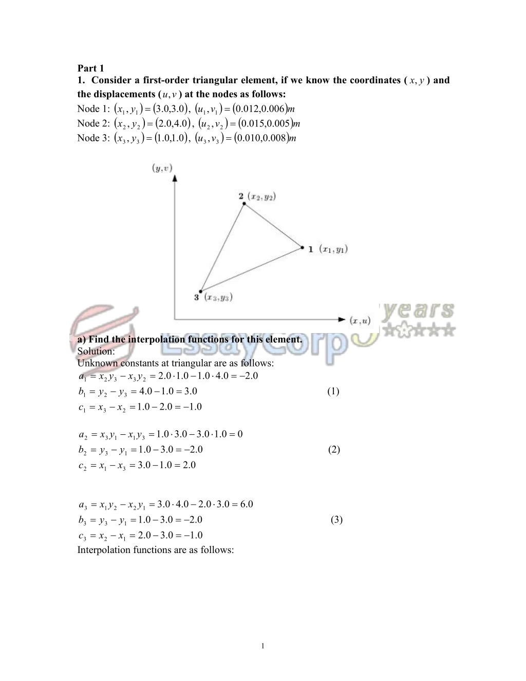
Part 1 1. Consider a first-order triangular element, if we know the coordinates ( the displacements ( v u, ) at the nodes as follows: Node 1: 0 . 3 , 0 . 3 , 1 1 y x v u . 0 , 1 1 Node 2: 0 . 4 , 0 . 2 , 2 2 y x v u . 0 , 2 2 Node 3: 0 . 1 , 0 . 1 , 3 3 y x v u . 0 , 3 3 ) and x, y , , , m 012 006 005 . 0 , 015 . 0 , 010 . 0 , m m 008 a) Find the interpolation functions for this element. Solution: Unknown constants at triangular are as follows: 0 . 1 0 . 2 2 3 3 2 1 y x y x a 0 . 3 0 . 1 0 . 4 3 2 1 y y b 0 . 1 0 . 2 0 . 1 2 3 1 x x c 0 . 1 0 . 4 0 . 2 (1) y x 0 . 1 0 . 3 0 . 1 0 . 3 0 . 3 0 . 2 0 . 2 0 . 1 a b c x y x y x y 0 . 1 0 . 3 0 2 3 1 1 3 (2) 2 3 1 2 1 3 y x 0 . 4 0 . 3 a b c Interpolation functions are as follows: x y x y x y 0 . 3 0 . 3 0 . 3 0 . 2 0 . 6 3 1 2 2 1 0 . 2 0 . 1 (3) 0 . 1 0 . 2 3 3 1 3 2 1 1
1 N N x , y a b x c y 1 1 1 1 1 1 2 (4) N N x , y a b x c y 2 2 2 2 2 1 2 N N x , y a b x c y 3 3 3 3 3 2 1 x y 1 0 . 3 0 . 3 1 1 1 1 where 1 x y 1 0 . 2 0 . 4 0 . 4 2 2 2 2 1 x y 1 0 . 1 0 . 1 3 3 1 1 N a b x c y 0 . 2 0 . 3 x y 1 1 1 1 2 8 1 1 (5) N a b x c y 0 . 2 x 2 y 2 2 2 2 2 8 1 1 0 . 6 N a b x c y 0 . 2 x y b) Calculate the displacements In triangular element, displacement approach is as follows: 3 u N u N u N u i 3 v N v N v N v i At the point 3 , 4 , interpolation functions are 1 0 . 2 0 . 6 8 From Eq.(6), (7) and (8), displacements at point 3 , 4 u At the point 2 , 3 , interpolation functions are 2 0 . 2 0 . 6 0 . 6 8 Similarly, from Eq.(6), (7) and (9), displacements at point 2 , 3 u 2. Determine the transformation equations and Jacobian matrix for the element given below. 3 3 3 3 2 8 v at the points 3 , 4 and 2 , 3 u, (6) N u i i 1 1 2 2 3 3 1 (7) N v i i 1 1 2 2 3 3 1 1 1 7 N 0 . 2 0 . 3 x y 0 . 2 0 . 3 0 . 4 0 . 3 1 8 8 8 1 1 1 (8) N 0 . 2 x 2 y 0 . 2 0 . 4 0 . 2 0 . 3 2 8 8 4 1 5 0 . 6 N x y 0 . 2 0 . 4 0 . 3 3 8 8 3 , 4 are . 0 , v . 0 0005 3 , 4 001 1 5 N 0 . 2 0 . 9 0 . 2 1 8 8 1 2 (9) N 0 . 6 0 . 4 2 8 8 1 N 3 8 2 , 3 are , v . 0 00125 2 , 3 . 0 0005 2
Local node number 1 2 3 4 5 6 7 8 i i -2.5 1.5 6.5 5.5 4.5 -0.5 -6.5 -4.5 -4 -4 -4 0 4 4 4 0 1 1 For vertex nodes 1,3,5,7, functions are . N 1 1 i i i i i 4 Therefore, 1 1 (10) N 1 5 . 2 1 4 5 . 2 4 1 4 1 1 (11) N 1 5 . 6 1 4 5 . 6 4 3 4 1 1 (12) N 1 5 . 4 1 4 5 . 4 4 5 4 1 1 5 . 6 5 . 6 (13) N 1 1 4 4 7 4 2 i 2 i 2 2 For midside nodes 2,4,6,8, functions are . N 1 1 1 1 i i i 2 2 Therefore, . 2 25 16 5 . 1 2 2 (14) N 1 1 1 4 1 2 2 2 3
30 . 25 5 . 5 2 (15) N 1 1 4 2 . 0 25 16 5 . 0 2 2 (16) N 1 1 1 4 1 6 2 2 20 . 25 2 (17) N 1 5 . 4 1 8 2 Transformation equations are as follows; i i Inserting Eqs. (10)-(17) into (18) and (19), the transformation equations of this element is obtained. Given the transformations, Jocobian can be obtained according the following Eq. (20) y x 8 (18) x N , x i i 8 1 (19) y N , y i i 1 x y (20) J Part 2 Plane Elasticity in Finite Element Analysis Gusset plates are commonly used to connect beams and columns in various structures. They can be fastened either by bolts or rivets. A cross gusset plate is shown in Figure 1. There are four bolting holes on the plate. When in service, four bolts are fitted in these holes. Loads of 20kN and 10 kN are applied on the bolts in horizontal and vertical directions, respectively. The cross gusset plate is made of mild steel with a thickness of 0.005 m. The stress-strain curve of the mild steel is shown in Figure 2. 1. Build a 2-D symmetric FE model using Abaqus to study the static response of the cross gusset plate under loading, including a mesh convergence analysis. (Note: You are required to define your geometry within Abaqus for this assignment) 2. Writing report on your FEA following the guidelines below. 4
Figure 1. Cross gusset technical drawing and applied loads resultant from bolting (all units are given in meters) Solution: 1) Brief 5
1/4 symmetry model for Finite element analysis Boundary and loading conditions 6
At 1/4 symmetric model, x-displacement of nodes on left vertical edge is fixed and y- displacement of nodes on horizontal edge is fixed. Loads of 10KN and 20KN on a end points of both circles is applied. FEA result (von-Misses stress distribution) 2) FEA procedures at commercial finite element analysis program ABAQUS - Geometric profile making 7
- Material and section definition - Assignment of material and section 8
- Definition of Assembly - Definition of static step 9
- Definition of boundary condition On bottom edge; On left vertical edge; 10
-Definition of loading - Submission of simulation process 11