Download

1 / 50
500 likes | 673 Views
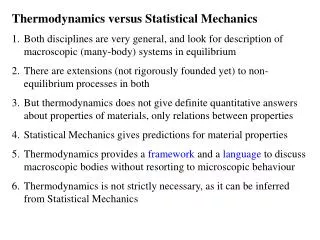
Statistical Mechanics of the Climate System. Valerio Lucarini valerio.lucarini@zmaw.de Meteorologisches Institut , Klimacampus , University of Hamburg Dept. of Mathematics and Statistics, University of Reading. Budapest,September 24 th 2013. A complex system: our Earth. Nonlinearity

E N D
Statistical Mechanics of the Climate System Valerio Lucarini valerio.lucarini@zmaw.de MeteorologischesInstitut, Klimacampus, University of Hamburg Dept. of Mathematics and Statistics, University of Reading Budapest,September 24th 2013
A complex system: our Earth Nonlinearity Irreversibility Disequilibrium Multiscale climate (Kleidon, 2011)
Looking for the big picture • Global structural properties: • Nonlinearity • Irreversibility • Disequilibrium • Multiscale • Stat Mech & Thermodynamic perspective • Planets are non-equilibrium thermodynamical systems • Thermodynamics: large scale properties of climate system; • Ergodic theory and much more • Stat Mech for Climate response to perturbations 3 EQ NON EQ
Features/Particles • Focus is on specific (self)organised structures • Hurricane physics/track
Atmospheric (macro) turbulence • Energy, enstrophy cascades, 2D vs 3D Note: NOTHING is really 2D in the atmosphere
Waves in the atmosphere • Large and small scale patterns
Motivations and Goals • What makes it so difficult to model the geophysical fluids? • Some gross mistakes in our models • Some conceptual/epistemological issues • What is a response? What is a parametrization? • Examples and open problems • Recent results of the perturbation theory for non-equilibrium statistical mechanics • Deterministic & Stochastic Perturbations • Applications on system of GFD interest • Lorenz 96 – various observables • Again: what is a parametrization? • Mori Zwanzig and Ruelle approaches • Try to convince you this is a useful framework even if I talk about a macro-system and the title of the workshop is …
Major theoreticalchallengesfor complex, non-equilibriumsystems • Mathematics: Stabilityprop of time mean state saynothing on the prop of the system • Cannotdefine a simpletheoryof the time-meanpropertiesrelyingonly on the time-meanfields. • Physics: “no” fluctuation-dissipationtheorem for a chaotic dissipative system • non-equivalence of external/ internalfluctuationsClimateChangeis hard to parameterise • Numerics: Complexsystemsfeaturemultiscaleproperties, they are stiffnumericalproblems, hard to simulate “asthey are”
Responsetheory • The response theory is a Gedankenexperiment: • a system, a measuring device, a clock, turnable knobs. • Changes of the statistical properties of a system in terms of the unperturbed system • Divergence in the response tipping points • Suitable environment for a climate change theory • “Blind” use of several CM experiments • We struggle with climate sensitivity and climate response • Deriving parametrizations!
Background • In quasi-equilibrium statistical mechanics, the Kubo theory (’50s) allows for an accurate treatment of perturbations to the canonical equilibrium state • In the linear case, the FDT bridges the properties of the forced and free fluctuations of the system • When considering general dynamical systems (e.g. forced and dissipative), the situation is more complicated (no FDT, in general) • Recent advances (Ruelle, mostly): for a class of dynamical systems it is possible to define a perturbativetheory of the response to small perturbations • We follow this direction… • We apply the theory also for stochastic forcings
Axiom A systems • Axiom A dynamical systems are very special • hyperbolic on the attractor • SRB invariant measure • time averages ensemble averages • Locally, “Cantor set times a smooth manifold” • Smoth on unstable (and neutral) manifold • Singular on stable directions (contraction!) • When we perform numerical simulations, we implicitly set ourselves in these hypotheses • Chaotic hypothesis by Gallavotti& Cohen (1995, 1996): systems with many d.o.f. can be treated as if they were Axiom A when macroscopic averages are considered. • These are, in some sense, good physical models!!!
Applicability of FDT • For deterministic, dissipative chaotic etc. systems FDT does not work • It is not possible to write the response as a correlation integral, there is an additional term • The system, by definition, never explores the stable directions, whereas a perturbations has components also outside the unstable manifold • Recent studies (Branstator et al.) suggest that, nonetheless, information can be retrieved • Probably, numerical noise also helps • The choice of the observable is surely also crucial • Parametrization
Ruelle (’98) Response Theory • Perturbed chaotic flow as: • Change in expectation value of Φ: • nthorderperturbation:
This is a perturbative theory… • with a causal Green function: • Expectation value of an operator evaluated over the unperturbed invariant measure ρSRB(dx) • where: and • Linear term: • Linear Green: • Linear suscept:
Kramers-Kronig relations • The in-phase and out-of-phase responses are connected by Kramers-Kronig relations: • Measurements of the real (imaginary) part of the susceptibility K-K imaginary (real) part • Every causal linear model obeys these constraints • K-K exist also for nonlinear susceptibilities with Kramers, 1926; Kronig, 1927
Linear Spectroscopy of L63 • Resonances have to do with UPOs
A Climate Change experiment • Observable: globally averaged TS • Forcing: increase of CO2 concentration • Linear response: • Let’s perform an ensemble of experiments • Concentration is increased at t=0 • Fantastic, we estimate • …and we obtain: • … we can predict future TS … In Progress…
Noise in Numerical Modelling • Deterministic numerical models are supplemented with additional stochastic forcings. • Overall practical goals: • an approximate but convincing representation of the spatial and temporal scales which cannot be resolved; • faster exploration of the attractor of the system, due to the additional “mixing”; • Especially desirable when computational limitations • Fundamental reasons: • A good (“physical”) invariant measure of a dynamical system is robust with respect to the introduction of noise • exclusion of pathological solutions; • Limit of zero noise → statistics of the deterministic system? • Noise makes the invariant measure smooth • A very active, interdisciplinary research sector
Stochastic forcing • , where is a Wiener process • Therefore, and • We obtain: • The linear correction vanishes; only even orders of perturbations give a contribution • No time-dependence
Some observations • The correction to the expectation value of any observable ~ variance of the noise • Stochastic system → deterministic system • Convergence of the statistical properties is fast • We have an explicit formula!
Correlations... • Ensemble average over the realisations of the stochastic processes of the expectation value of the time correlation of the response of the system: • Leading order is proportional to ε2 • It is the convolution product of the linear Green function!
So what? • Computing the Fourier Transform we obtain: • We end up with the linear susceptibility... • Let’s rewrite he equation: • So: difference between the power spectra • → square modulus of linear susceptibility • Stoch forcing enhances the Power Spectrum • Can be extended to general (very) noise • KK linear susceptibility Green function
With some complex analysis • We know that is analytic in the upper complex plane • So is • Apart from complex zeros... • The real ( ) and imag ( ) obey KK relations • From the observation of the power spectra we obtain the real part • With KK analysis we obtain the imaginary part • We can reconstruct the linear susceptibility! • And from it, the Green function
Lorenz 96 model • Excellent toy model of the atmosphere • Advection • Dissipation • Forcing • Test Bed for Data assimilation schemes • Becoming popular in the community of statistical physicists • Scaling properties of Lyapunov & Bred vectors • Evolution Equations • Spatially extended, 2 Parameters: N & F
Some properties • Let • and • Stationary State: • Closure: • System is extended, in chaotic regime the properties are intensive • We perform simulations with specific F=8 and N=40, but results are “universal”
Global Perturbation • Observable: e=E/N • We can compute the leading order for both the real and imaginary part L & Sarno, 2011
Imag part of the susceptibility LW HF Rigorous extrapolation
Real part of the susceptibility LW HF Rigorous extrapolation
Green Function! • Inverse FT of the susceptibility • Response to any forcing with the same spatial pattern but with general time pattern
Using stochastic forcing… • Squared modulus of • Blue: Using stoch pert; Black: deter forcing • ... And many many many less integrations
What is a Parametrization? • Surrogating the coupling: FastSlow Variables • Optimising Computer Resources • Underlining Mechanismsof Interaction • How to perform coarse-graining
Empirical Parametrization (Wilks ‘05) • Lorenz ‘96 model • Parametrization of Y’s • Deterministic + Stoch • Best Fit of residuals • Have to repeat for each model • Weak coupling
Traditionally… • Parametrizations obtained as empirical closure formulas • Vertical transport of momentum at the border of the boundary layer as a function of …. • Evaporation over ocean given …. • These formulas are deterministic functions of the larger scale variables • … or tables are used • Recently, people are proposing stochastic parametrizations in the hope of mimicking better the variability
Conditional Markov Chains (Crommelin et al.) • Data-inferred conditional Markov chains • U: unresolved dynamics; X: resolved variables • Construct from data a transition matrix • Strength of the unresolved dynamics given its strength at previous step and the values of the resolved variables at the present & previous steps • Discretization of the problem for the unresolved dynamics • Rules constructed from data memory • Works also for not-so-weak coupling
Systematic Mode Reduction (Majda et al.) • Fluid Dynamics Eqs (e.g. QG dynamics) • X: slow, large scale variables • Y: unresolved variables (EOF selection) • Ψ are quadratic • Conditions: • The dynamics of unresolved modes is ergodicand mixing • It can be represented by a stochastic process • all unresolved modes are quasi-Gaussian distributed • One can derive an effective equation for the X variables where is F is supplemented with: • A deterministic correction • An additive and a multiplicative noise
Problems • A lot of hypotheses • Impact of changing the forcing? • Impact of changing the resolution? • Parametrizationshould obey physical laws • If we perturb q and T, we should have LΔq=CpΔT • Energy and momentum exchange • Consistency with regard to entropy production… • The impact of stochastic perturbations can be very different depending on what variables are perturbed • Assuming a white noise can lead to large error • Planets!
How to Construct a Parametrization? • We try to match the evolution of the single trajectory of the X variables • Mori-Zwanzig Projector Operator technique: needs to be made explicit • Accurate “Forecast” • We try to match the statistical properties of a general observable A=A(X) • RuelleResponse theory • Accurate “Climate” • Match between these two approaches?
That’s the result! • This system has the same expectation values as the original system (up to 2nd order) • We have explicit expression for the three terms a (deterministic), b (stochastic), c (memory)- 2nd order expansion a b c T O D A Y Deterministic ✓ Stochastic ✓ Memory ✖
Diagrams: 1st and 2nd order • 1 • 2 Coupling Time +
Mean Field • Deterministic Parametrization • This is the “average” coupling
Fluctuations • Stochastic Parametrization • Expression for correlation properties
Memory • New term, small for vast scale separation • This is required to match local vs global
Two words on Mori-Zwanzig • Answers the following question • what is the effective X dynamics for an ensemble of initial conditions Y(0), when ρY is known? • We split the evolution operator using a projection operator P on the relevant variables • Effective dynamics has a deterministic correction to the autonomous equation, a term giving a stochastic forcings (due to uncertainty in the the initial conditions Y(0)), a term describing a memory effect. • One can perform an approximate calculation, expanding around the uncoupled solution…
Mori-Zwanzig: a simple example (Gottwald, 2010) • Just a 2X2 system: • x is “relevant” • We solve with respect to y: • We plug the result into x: • Markov Memory Noise
Same result! • Optimal forecast in a probabilistic sense • 2nd order expansion • Same as obtained with Ruelle • Parametrizations are “well defined” for CM & NWP a b c • Memory required to match local vs global
Conclusions • We have used Ruelleresponse theory to study the impact of deterministic and stochastic forcings to non-equilibrium statistical mechanical systems • Frequency-dependent response obeys strong constraints • We can reconstruct the Green function! • Δexpectation value of observable ≈variance of the noise • SRB measure is robust with respect to noise • Δ power spectral density ≈ to the squared modulus of the linear susceptibility • More general case: Δ power spectral density >0 • What is a parametrization? I hope I gave a useful answer • We have ground for developing new and robust schemes • Projection of the equations smooth measure FDT! • Application to more interesting models • TWO POST-DOC POSITIONS
References • D. Ruelle, Phys. Lett. 245, 220 (1997) • D. Ruelle, Nonlinearity 11, 5-18 (1998) • C. H. Reich, Phys. Rev. E 66, 036103 (2002) • R. Abramov and A. Majda, Nonlinearity 20, 2793 (2007) • U. Marini Bettolo Marconi, A. Puglisi, L. Rondoni, and A. Vulpiani, Phys. Rep. 461, 111 (2008) • D. Ruelle, Nonlinearity 22 855 (2009) • V. Lucarini, J.J. Saarinen, K.-E. Peiponen, E. Vartiainen: Kramers-Kronig Relations in Optical Materials Research, Springer, Heidelberg, 2005 • V. Lucarini, J. Stat. Phys. 131, 543-558 (2008) • V. Lucarini, J. Stat. Phys. 134, 381-400 (2009) • V. Lucarini and S. Sarno, Nonlin. Proc. Geophys. 18, 7-27 (2011) • V. Lucarini, T. Kuna, J. Wouters, D. Faranda, Nonlinearity (2012) • V. Lucarini, J. Stat. Phys. 146, 774 (2012) • J. Wouters and V. Lucarini, J. Stat. Mech. (2012) • J. Wouters and V. Lucarini, J Stat Phys. 2013 (2013)