Download
1 / 61
640 likes | 860 Views
Constraint Satisfaction Problems. Chapter 5. In which we see how treating states as more than just little black boxes leads to the invention of a range of powerful new search methods and a deeper understanding of problem structure and complexity.

E N D
Constraint Satisfaction Problems Chapter 5
In which we see how treating states as more than just little black boxes leads to the invention of a range of powerful new search methods and a deeper understanding of problem structure and complexity. • Allows useful general-purpose algorithms with more power than standard search algorithms
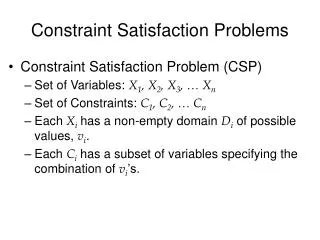
Constraint satisfaction problems (CSPs) • A constraint satisfaction problem (or CSP) is defined by: • a set of variables, X1, X2,…, Xn, and • a set of constraints, C1, C2,…, Cm. • Each variable Xihas a nonempty domain Diof possible values. • Each constraint Ciinvolves some subset of the variables and specifies the allowable combinations of values for that subset. • We will focus on binary constraints, i.e. subsets of two vars • An assignment that does not violate any constraints is called a consistent or legal assignment. • A complete assignment is one in which every variable is mentioned, and a solution to a CSP is a complete assignment that satisfies all the constraints.
Example: Map-Coloring • VariablesWA, NT, Q, NSW, V, SA, T • DomainsDi = {red, green, blue} • Constraints: adjacent regions must have different colors • e.g., WA ≠ NT, • or (WA,NT) in {(red,green),(red,blue),(green,red),(green,blue),(blue,red),(blue,green)}
Constraint graph • Binary CSP: each constraint relates two variables • Constraint graph: nodes are variables, arcs are constraints
CSP as a search problem • State: is defined by an assignment of variablesXi with values from domainDi • Initial state: the empty assignment {}, in which all variables are unassigned. • Successor function: a value can be assigned to any unassigned variable, provided that it does not conflict with previously assigned variables. • Goal test:the current assignment is complete. I.e. all variables are assigned values complying to the set of constraints • Path cost:a constant cost (e.g., 1) for every step.
CSP as a search problem (cont.) • Every solution must be a complete assignment and therefore appears at depth nif there are nvariables. • Furthermore, the search tree extends only to depth n. • For these reasons, depth-first search algorithms are popular for CSP’s. • It is also the case that the path by which a solution is reached is irrelevant.
Example: Map-Coloring • Solutions are complete and consistent assignments, e.g., • WA = red, NT = green, Q = red, NSW = green, V = red, SA = blue, T = green
Varieties of constraints • Unary constraints involve a single variable, • e.g., SA ≠ green • can be dealt with by filtering the domain of involved variables • Binary constraints involve pairs of variables, • e.g., SA ≠ WA • Higher-order constraints involve 3 or more variables
Standard search formulation (incremental) Let’s try a classical search on a CSP. Suppose |D1| = |D2| =…= |Dn| = d Something terrible: the branching factor at the top level is n*d, because any of dvalues can be assigned to any of nvariables. At the next level, the branching factor is (n-1)*d (In the worst case, e.g. when there aren’t constraints at all) … We generate a tree with n!*dn leaves although there are dn possible assignments!
Backtracking search • Variable assignments are commutative, i.e., [WA = red then NT = green] same as [NT = green then WA = red] • So, we only need to consider assignments to a single variable at each node b = d and there are dn leaves (Again, in the worst case, e.g. when there aren’t constraints at all) • Depth-first search for CSP ’s with single-variable assignments is called backtracking search • Backtracking search is the basic algorithm for CSP ’s • Recall, we are looking for any solution, since all the solutions are at the same depth and hence the same cost. • Now, by picking a good order to try the variables, we can drastically avoid to explore all the above search tree with dn leaves.
Depth-First Search on CSP The fringe will be implemented by a stack. We also change the terminology a bit: problem = csp node = assignment initialstate = {}//empty assignment is initial state DFS-Search(csp, fringe) assignment = MakeNode({}); Insert(fringe, assignment); do if ( Empty(fringe) ) return failure; assignment = Remove(fringe); if ( assignment is complete ) return assignment; InsertAll (fringe, Expand(assignment, csp) ); while (true);
A closer look at Expand(assignment, csp) • To expand an assignment means to assign a value at an unassigned yet variable and complying to the constraints. • Which unassigned variable we pick for assignment turns out to be very important in quickly finding a solution. • Also, the order of values we pick from the domain to assign to the picked variable is important. • In other words, the order of the list of successors returned by Expand(…) is very important in quickly finding a solution. • In the next slide, we show a recursive version of DFS, where the above mentioned orders are more explicit.
Improving backtracking efficiency • Plain backtracking is an uninformed algorithm in the terminology of Chapter 3, so we do not expect it to be very effective for large problems. • In Chapter 4, we remedied the poor performance of uninformed search algorithms by supplying them with domain-specific heuristic functions derived from our knowledge of the problem. • It turns out that we can solve CSPs efficiently without such domain-specific knowledge. • General-purpose methods can give huge gains in speed. • Such methods address the following questions: • Which variable should be assigned next? • In what order should its values be tried? • Can we detect inevitable failure early?
Variable and value ordering • The backtracking algorithm contains the line • By default, it simply selects the next unassigned variable in the order given by the list VARIABLES[csp]. • This seldom results in the most efficient search. • For example, after the assignments for WA=redand NT =green, there is only one possible value for SA, so it makes sense to assign SA=bluenext rather than assigning Q. • In fact, after SAis assigned, the choices for Q, NSW, and Vare all forced.
Variable and value ordering • This intuitive idea—choosing the variable with the fewest “legal” values—is called the minimum remaining values (MRV) heuristic. • It also has been called the “most constrained variable” or “fail-first” heuristic, because it picks a variable that is most likely to cause a failure soon, thereby pruning the search tree. • If there is a variable Xwith zero legal values remaining, the MRV will select Xand failure will be detected immediately—avoiding pointless searches through other variables which always will fail when Xis finally selected.
Most constrained variable • Most constrained variable: choose the variable with the fewest legal values • minimum remaining values (MRV) heuristic
Degree Heuristic • The MRV heuristic doesn’t help at all in choosing the first region to color in Australia, • because initially every region has three legal colors. • In this case, the degree heuristic comes in handy. It attempts to reduce the branching factor on future choices by selecting the variable that is involved in the largest number of constraints on other unassigned variables. • Not only the first time: The MRV heuristic is usually a more powerful guide, but the degree heuristic can be useful as a tie-breaker.
Least constraining value • Once a variable has been selected, the algorithm must decide on the order in which to examine its values. • For this, the least-constraining-value heuristic can be effective. • It prefers the value that rules out the fewest choices for the neighboring variables in the constraint graph.
Forward checking • Idea: • Keep track of remaining legal values for unassigned variables • Terminate search when any variable has no legal values
Forward checking • Idea: • Keep track of remaining legal values for unassigned variables • Terminate search when any variable has no legal values
Forward checking • Idea: • Keep track of remaining legal values for unassigned variables • Terminate search when any variable has no legal values
Forward checking • Idea: • Keep track of remaining legal values for unassigned variables • Terminate search when any variable has no legal values
Constraint propagation • Forward checking propagates information from assigned to unassigned variables, but doesn't provide early detection for all failures: • E.g. NT and SA cannot both be blue! • Constraint propagation repeatedly enforces constraints locally
Arc consistency • Simplest form of propagation makes each arc () consistent. • Here, “arc” refers to a directed arc in the constraint graph, such as the arc from SAto NSW. • An arc X Y is consistent iff for every value x of X there is some allowed value y of Y
Arc consistency • Simplest form of propagation makes each arc consistent • X Y is consistent iff for every value x of X there is some allowed y
Arc consistency • Simplest form of propagation makes each arc consistent • X Y is consistent iff for every value x of X there is some allowed y • If X loses a value, neighbors of X need to be rechecked
Arc consistency • Simplest form of propagation makes each arc consistent • X Y is consistent iff for every value x of X there is some allowed y • If X loses a value, neighbors of X need to be rechecked • Arc consistency detects failure earlier than forward checking • Can be run as a preprocessor or after each assignment
Class Problem – AC-3 • AC-3 algorithm can detect the inconsistency of the partial assignment {WA=red; V =blue}. • Queue = {QNT,…,SAWA, NTWA, SAV,NSWV} • Only the last 4 are inconsistent. All the arcs before those will be dequeued and thrown away, since they aren’t incons. • Dequeueing SAWA: inconsistent, remove red from SA. Insert NTSA, QSA, NSWSA, VSA in the queue. • Dequeueing NTWA: inconsistent, remove red from NT. Insert QNT, SANT, WANT in the queue. • Dequeueing SAV: inconsistent, remove blue from SA leaving only green. Insert VSA, NSWSA, QSA, NTSA • Dequeueing NSWV: inconsistent, remove blue from NSW. Insert SANSW, QNSW, VNSW • Dequeueing NTSA: consistent
Class Problem – AC-3 • Dequeueing QSA: inconsistent, remove green from Q. Insert NSWQ, SAQ, NTQ • Dequeueing VSA: consistent • Dequeueing NSWSA: inconsistent, remove green from NSW leaving only red. Insert SANSW, QNSW, VNSW • Dequeueing QSA, NTSA, SANSW, QNSW, VNSW: consistent • Dequeueing NSWQ: inconsistent removing red from Q leaving only blue. Insert NTQ, … • Dequeueing SAQ, NTQ, SANSW, QNSW, VNSW: consistent • Dequeueing NTQ removing blue from NT leaving only green. Insert WANT, SANT, … • Dequeueing …SAQ: inconsistent removing green from SA, leaving no color for SA.
Complexity of arc consistency • The complexity of arc consistency checking can be analyzed as follows: • a binary CSP has at most O(n2)arcs; • each arc (Xk,Xi)can be inserted on the agenda only dtimes, because Xihas at most dvalues to delete; • checking consistency of an arc can be done in O(d2)time; • so the total worst-case time is O(n2d3).
Local search for CSPs • Hill-climbing, simulated annealing typically work with "complete" states, i.e., all variables assigned • To apply to CSPs: • allow states with unsatisfied constraints • operators reassign variable values • Variable selection: randomly select any conflicted variable • Value selection by min-conflicts heuristic: • choose value that violates the fewest constraints • i.e., hill-climb with h(n) = total number of violated constraints
Summary • CSPs are a special kind of problem: • states defined by values of a fixed set of variables • goal test defined by constraints on variable values • Backtracking = depth-first search with one variable assigned per node • Variable ordering and value selection heuristics help significantly • Forward checking prevents assignments that guarantee later failure • Constraint propagation (e.g., arc consistency) does additional work to constrain values and detect inconsistencies • Iterative min-conflicts is usually effective in practice
Class Problem – Crossword Puzzles • Consider the problem of constructing (not solving) crossword puzzles: fitting words into a rectangular grid. • The grid, which is given as part of the problem, specifies which squares are blank and which are shaded. • Assume that a list of words (i.e., a dictionary) is provided. • Formulate this problem as a constraint satisfaction problem.
Class Problem – Crossword Puzzles • Variables: one for each line, and one for each column. • H1, H2, H3, H4, H5 • V1, V2, V3, V4, V5, V6 • Domains: Subsets of English words, • E.g. DH2 is the set of all 5-letter English words. • Constraints: One constraint between each two variables that intersect • E.g. H1V2 saying that H1[2] = V2[1] V1 V2 V3 V4 V5 V6 H1 H2 H3 H4 H5
Class Problem – Rectilinear floor-planning: • Problem: Find non-overlapping places in a large rectangle for a number of smaller rectangles. • Let’s assume that the floor is a grid. • Variables: one for each of the small rectangles, • with the value of each variable being a 4tuple consisting of the coordinates of the upper left and lower right corners of the place where the rectangle will be located. • Domains: for each variable it is the set of 4tuples that are the right size for the corresponding small rectangle and that fit within the large rectangle. • Constraints: say that no two rectangles can overlap; • E.g. if the value of variable X1 is [0,0,5,8], then no other variable can take on a value that overlaps with the [0,0,5,8] rectangle.
Class Problem – Class-Scheduling • There is a fixed number of professors and classrooms, a list of classes to be offered, and a list of possible time slots for classes. Each professor has a set of classes that he or she can teach. • Variables: One for each class. • Values are triples (classroom, time, professor) • Domains: For each variable Ci we set Di as the set of all the possible triples after filtering out those triples with third element a professor that doesn’t teach Ci. • Constraints: one for each pair of variables (Ci Cj) saying: • !(classroomi == classroomj && timei==timej) • !(professori == professorj && timei==timej)
Class Problem – Zebra • Consider the following logic puzzle: In five houses, each with a different color, live 5 persons of different nationalities, each of whom prefer a different brand of cigarette, a different drink, and a different pet. Given the following facts, the question to answer is • “Where does the zebra live, and in which house do they drink water?”
Class Problem – Zebra The Englishman lives in the red house. The Spaniard owns a dog. Coffee is drunk in the green house. The Ukrainian drinks tea. The green house is directly to the right of the ivory house. The Old-Gold smoker owns snails. Kools are being smoked in the yellow house. Milk is drunk in the middle house. The Norwegian lives in the first house on the left. The Chesterfield smoker lives next to the fox owner. Kools are smoked in the house next to the house where the horse is kept. The Lucky-Strike smoker drinks orange juice. The Japanese smokes Parliament. The Norwegian lives next to the blue house.
Class Problem - Zebra • Variables: five variables for each house, one with the domain of colors, one with pets, and so on. Total 25 variables. I.e. • color1, …, color5, • drink1, …, drink5 • nationality1, …, nationality5 • pet1, …, pet5 • cigarette1, …, cigarette5 • Domains: • Blue, Green, Ivory, Red, Yellow • Coffee, Milk, Orange, Juice, Tea, Water • Englishman, Japanese, Norwegian, Spaniard, Ukrainian • Dog, Fox, Horse, Snails, Zebra • Chesterfield, Kools, Lucky-Strike, Old-Gold, Parliament
Class Problem - Zebra • Constraints: • Unary: Rules 8 (Milk is drunk in the middle house) and 9 (The Norwegian lives in the first house on the left): • drink3=Milk • nationality1=Norwegian • We filter the corresponding domains