Constraint Satisfaction Problems

Constraint Satisfaction Problems Slides by Prof WELLING

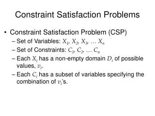
Constraint satisfaction problems (CSPs) • CSP: • state is defined by variablesXi with values from domainDi • goal test is a set of constraints specifying allowable combinations of values for subsets of variables • Allows useful general-purpose algorithms with more power than standard search algorithms

Example: Map-Coloring • VariablesWA, NT, Q, NSW, V, SA, T • DomainsDi = {red,green,blue} • Constraints: adjacent regions must have different colors • e.g., WA ≠ NT

Example: Map-Coloring • Solutions are complete and consistent assignments, e.g., WA = red, NT = green,Q = red,NSW = green,V = red,SA = blue,T = green

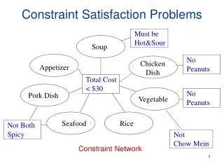
Constraint graph • Binary CSP: each constraint relates two variables • Constraint graph: nodes are variables, arcs are constraints

Varieties of CSPs • Discrete variables • finite domains: • n variables, domain size d  O(d n) complete assignments • e.g., 3-SAT (NP-complete) • infinite domains: • integers, strings, etc. • e.g., job scheduling, variables are start/end days for each job: StartJob1 + 5 ≤ StartJob3 • Continuous variables • e.g., start/end times for Hubble Space Telescope observations • linear constraints solvable in polynomial time by linear programming

Varieties of constraints • Unary constraints involve a single variable, • e.g., SA ≠ green • Binary constraints involve pairs of variables, • e.g., SA ≠ WA • Higher-order constraints involve 3 or more variables, • e.g., SA ≠ WA ≠ NT

Example: Cryptarithmetic • Variables: F T U W R O X1 X2 X3 • Domains: {0,1,2,3,4,5,6,7,8,9} {0,1} • Constraints: Alldiff (F,T,U,W,R,O) • O + O = R + 10 ·X1 • X1 + W + W = U + 10 · X2 • X2 + T + T = O + 10 · X3 • X3 = F, T ≠ 0, F≠ 0

Real-world CSPs • Assignment problems • e.g., who teaches what class • Timetabling problems • e.g., which class is offered when and where? • Transportation scheduling • Factory scheduling • Notice that many real-world problems involve real-valued variables

NxD WA WA WA NT T [NxD]x[(N-1)xD] WA NT WA NT WA NT NT WA Standard search formulation • Let’s try the standard search formulation. • We need: • Initial state: none of the variables has a value (color) • Successor state: one of the variables without a value will get some value. • Goal: all variables have a value and none of the constraints is violated. N layers Equal! N! x D^N There are N! x D^N nodes in the tree but only D^N distinct states??

NT WA WA NT = Backtracking (Depth-First) search • Special property of CSPs: They are commutative: • This means: the order in which we assign variables • does not matter. • Better search tree: First order variables, then assign them values one-by-one. D WA WA WA WA NT D^2 WA NT WA NT D^N

Backtracking example

Improving backtracking efficiency • General-purpose methods can give huge gains in speed: • Which variable should be assigned next? • In what order should its values be tried? • Can we detect inevitable failure early? • We’ll discuss heuristics for all these questions in the following.

Which variable should be assigned next?minimum remaining values heuristic • Most constrained variable: choose the variable with the fewest legal values • a.k.a. minimum remaining values (MRV) heuristic • Picks a variable which will cause failure as soon as possible, allowing the tree to be pruned.

Which variable should be assigned next? degree heuristic • Tie-breaker among most constrained variables • Most constraining variable: • choose the variable with the most constraints on remaining variables (most edges in graph)

In what order should its values be tried?  least constraining value heuristic • Given a variable, choose the least constraining value: • the one that rules out the fewest values in the remaining variables • Leaves maximal flexibility for a solution. • Combining these heuristics makes 1000 queens feasible

Rationale for MRV, DH, LCV • In all cases we want to enter the most promising branch, but we also want to detect inevitable failure as soon as possible. • MRV+DH: the variable that is most likely to cause failure in a branch is assigned first. E.g X1-X2-X3, values is 0,1, neighbors cannot be the same. • LCV: tries to avoid failure by assigning values that leave maximal flexibility for the remaining variables.

Can we detect inevitable failure early?  forward checking • Idea: • Keep track of remaining legal values for unassigned variables that are connected to current variable. • Terminate search when any variable has no legal values

Forward checking • Idea: • Keep track of remaining legal values for unassigned variables • Terminate search when any variable has no legal values

Constraint propagation • Forward checking only looks at variables connected to current value in constraint graph. • NT and SA cannot both be blue! • Constraint propagation repeatedly enforces constraints locally

Arc consistency • Simplest form of propagation makes each arc consistent • X Y is consistent iff for every value x of X there is some allowed y consistent arc. constraint propagation propagates arc consistency on the graph.

Arc consistency • Simplest form of propagation makes each arc consistent • X Y is consistent iff for every value x of X there is some allowed y inconsistent arc. remove blue from source consistent arc.

Arc consistency • Simplest form of propagation makes each arc consistent • X Y is consistent iff for every value x of X there is some allowed y • If X loses a value, neighbors of X need to be rechecked: i.e. incoming arcs can become inconsistent again (outgoing arcs will stay consistent). this arc just became inconsistent

Arc consistency • Simplest form of propagation makes each arc consistent • X Y is consistent iff for every value x of X there is some allowed y • If X loses a value, neighbors of X need to be rechecked • Arc consistency detects failure earlier than forward checking • Can be run as a preprocessor or after each assignment • Time complexity: O(n2d3)

Arc Consistency • This is a propagation algorithm. It’s like sending messages to neighbors on the graph! How do we schedule these messages? • Every time a domain changes, all incoming messages need to be re-send. Repeat until convergence  no message will change any domains. • Since we only remove values from domains when they can never be part of a solution, an empty domain means no solution possible at all  back out of that branch. • Forward checking is simply sending messages into a variable that just got its value assigned. First step of arc-consistency.

Try it yourself [R,B,G] [R,B,G] [R] [R,B,G] [R,B,G] Use all heuristics including arc-propagation to solve this problem.

B G R R G B a priori constrained nodes B R G B G B R G G R B Note: After the backward pass, there is guaranteed to be a legal choice for a child note for any of its leftover values. This removes any inconsistent values from Parent(Xj), it applies arc-consistency moving backwards.

Junction Tree Decompositions

Local search for CSPs • Note: The path to the solution is unimportant, so we can apply local search! • To apply to CSPs: • allow states with unsatisfied constraints • operators reassign variable values • Variable selection: randomly select any conflicted variable • Value selection by min-conflicts heuristic: • choose value that violates the fewest constraints • i.e., hill-climb with h(n) = total number of violated constraints

Example: 4-Queens • States: 4 queens in 4 columns (44 = 256 states) • Actions: move queen in column • Goal test: no attacks • Evaluation: h(n) = number of attacks

Summary • CSPs are a special kind of problem: • states defined by values of a fixed set of variables • goal test defined by constraints on variable values • Backtracking = depth-first search with one variable assigned per node • Variable ordering and value selection heuristics help significantly • Forward checking prevents assignments that guarantee later failure • Constraint propagation (e.g., arc consistency) does additional work to constrain values and detect inconsistencies • Iterative min-conflicts is usually effective in practice

Constraint Satisfaction Problems

Constraint Satisfaction Problems

Presentation Transcript