Download
1 / 12
120 likes | 228 Views
HowTo 03: stimulus timing design (hands-on). Goal: to design an effective random stimulus presentation end result will be stimulus timing files example: using an event related design, with simple regression to analyze Steps:

E N D
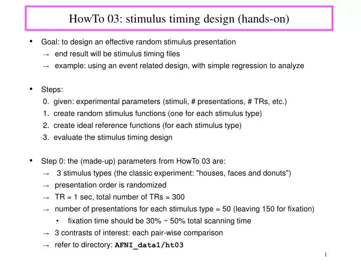
HowTo 03: stimulus timing design (hands-on) • Goal: to design an effective random stimulus presentation • end result will be stimulus timing files • example: using an event related design, with simple regression to analyze • Steps: 0. given: experimental parameters (stimuli, # presentations, # TRs, etc.) 1. create random stimulus functions (one for each stimulus type) 2. create ideal reference functions (for each stimulus type) 3. evaluate the stimulus timing design • Step 0: the (made-up) parameters from HowTo 03 are: • 3 stimulus types (the classic experiment: "houses, faces and donuts") • presentation order is randomized • TR = 1 sec, total number of TRs = 300 • number of presentations for each stimulus type = 50 (leaving 150 for fixation) • fixation time should be 30% ~ 50% total scanning time • 3 contrasts of interest: each pair-wise comparison • refer to directory: AFNI_data1/ht03
Step 1: creation of random stimulus functions • RSFgen : Random Stimulus Function generator • command file: c01.RSFgen RSFgen -nt 300 -num_stimts 3 \ -nreps 1 50 -nreps 2 50 -nreps 3 50 \ -seed 1234568 -prefix RSF.stim.001. • This creates 3 stimulus timing files: RSF.stim.001.1.1D RSF.stim.001.2.1D RSF.stim.001.3.1D • Step 2: create ideal response functions (linear regression case) • waver: creates waveforms from stimulus timing files • effectively doing convolution • command file: c02.waver waver -GAM -dt 1.0 -input RSF.stim.001.1.1D • this will output (to the terminal window) the ideal response function, by convolving the Gamma variate function with the stimulus timing function • output length allows for stimulus at last TR (= 300 + 13, in this example) • use '1dplot' to view these results, command: 1dplot wav.*.1D
the first curve (for wav.hrf.001.1.1D) is displayed on the bottom • x-axis covers 313 seconds, but the graph is extended to a more "round" 325 • y-axis happens to reach 274.5, shortly after 3 consecutive type-2 stimuli • the peak value for a single curve can be set using the -peak option in waver • default peak is 100 • it is worth noting that there are no duplicate curves • can also use 'waver -one' to put the curves on top of each other
Step 3: evaluate the stimulus timing design • use '3dDeconvolve -nodata': experimental design evaluation • command file: c03.3dDeconvolve • command: 3dDeconvolve -nodata \ -nfirst 4 -nlast 299 -polort 1 \-num_stimts 3 \-stim_file 1 "wav.hrf.001.1.1D" \-stim_label 1 "stim_A" \-stim_file 2 "wav.hrf.001.2.1D" \-stim_label 2 "stim_B" \-stim_file 3 "wav.hrf.001.3.1D" \-stim_label 3 "stim_C" \-glt 1 contrasts/contrast_AB \-glt 1 contrasts/contrast_AC \-glt 1 contrasts/contrast_BC
Use the 3dDeconvolve output to evaluate the normalized standard deviations of the contrasts. • For this HowTo script, the deviations of the GLT's are summed. Other options are valid, such as summing all values, or just those for the stimuli, or summing squares. • Output (partial): Stimulus: stim_A h[ 0] norm. std. dev. = 0.0010 Stimulus: stim_B h[ 0] norm. std. dev. = 0.0009 Stimulus: stim_C h[ 0] norm. std. dev. = 0.0011 General Linear Test: GLT #1 LC[0] norm. std. dev. = 0.0013 General Linear Test: GLT #2 LC[0] norm. std. dev. = 0.0012 General Linear Test: GLT #3 LC[0] norm. std. dev. = 0.0013 • What does this output mean? • What is norm. std. dev.? • How does this compare to results using different stimulus timing patterns?
Basics about Regression • Regression Model (General Linear System) • Simple Regression Model (one regressor): Y(t) = a0+a1t+b r(t)+e(t) • Run 3dDeconvolve with regressor r(t), atime series IRF • Deconvolution and Regression Model (one stimulus with a lag of p TR’s): Y(t) = a0+a1t+b0f(t)+b1f(t-TR)…+bpf(t-p*TR)+e(t) • Run 3dDeconvolve with stimulus files (containing 0’s and 1’s) • Model in Matrix Format: Y = Xb + e • X: design matrix - more rows (TR’s) than columns (baseline parameters + beta weights). a0 a1 ba0 a1 b0 … bp ------------------ ------------------------ 1 1 r(0) 1 pfp … f0 1 2 r(1)1 p+1 fp+1… f1 . . . . . . 1 N-1 r(N-1)1 N-1 fN-1 … fN-p-1 • e: random (system) error N(0, s2)
X matrix examples (based on modified HowTo 03 script, stimulus #3): • regression: baseline, linear drift, 1 regressor (ideal response function) • deconvolution: baseline, linear drift, 5 regressors (lags) • decide on appropriate values of: a0 a1 bi Y regression deconvolution - with lags (0-7) a0a1b0a0 a1 b0 b1 b2 b3 b4 b5 b6 b7 500 1 0 0 1 0 0 0 0 0 0 0 0 0 500 1 1 0 1 1 1 0 0 0 0 0 0 0 500.01 1 2 0.1 1 2 1 1 0 0 0 0 0 0 500.91 1 3 9.1 1 3 0 1 1 0 0 0 0 0 505.60 1 4 56.0 1 4 0 0 1 1 0 0 0 0 513.69 1 5 136.9 1 5 0 0 0 1 1 0 0 0 518.82 1 6 188.2 1 6 0 0 0 0 1 1 0 0 517.42 1 7 174.2 1 7 1 0 0 0 0 1 1 0 512.19 1 8 121.9 1 8 0 1 0 0 0 0 1 1 507.81 1 9 78.1 1 9 0 0 1 0 0 0 0 1 508.06 1 10 80.6 1 10 1 0 0 1 0 0 0 0 510.44 1 11 104.4 1 11 0 1 0 0 1 0 0 0 511.29 1 12 112.9 1 12 0 0 1 0 0 1 0 0 512.49 1 13 124.9 1 13 1 0 0 1 0 0 1 0 513.64 1 14 136.4 1 14 0 1 0 0 1 0 0 1 513.06 1 15 130.6 1 15 0 0 1 0 0 1 0 0 513.32 1 16 133.2 1 16 0 0 0 1 0 0 1 0 513.98 1 17 139.8 1 17 0 0 0 0 1 0 0 1
Y e X-Space r1 • Solving the Linear System : Y = Xb + e • the basic goal of 3dDeconvolve • Least Square Estimate (LSE): making sum of squares of residual (unknown/unexplained) error e’e minimal Normal equation: (X’X) b = X’Y • When X is of full rank (all columns are independent), b^ = (X’X)-1X’Y • Geometric Interpretation: • project vector Y onto a space spanned by the regressors (the column vectors of design matrix X) • find shortest distance from Y to X-space Xb 0 r2
Multicollinearity Problem • 3dDeconvolve Error: Improper X matrix (cannot invert X’X) • X’Xis singular (not invertible) ↔at least one column of X is linearly dependent on the other columns • normal equation has no unique solution • Simple regression case: • mistakenly provided at least two identical regressor files, or some inclusive regressors, in 3dDeconvolve • all regressiors have to be orthogonal (exclusive) with each other • easy to fix: use 1dplot to diagnose • Deconvolution case: • mistakenly provided at least two identical stimulus files, or some inclusive stimuli, in 3dDeconvolve • easy to fix: use 1dplot to diagnose • intrinsic problem of experiment design: lack of randomness in the stimuli • varying number of lags may or may not help. • running RSFgen can help to avoid this • see AFNI_data1/ht03/bad_stim/c20.bad_stim
Design analysis • X’Xinvertible but cond(X’X) is huge linear system is sensitive difficult to obtain accurate estimates of regressor weights • Condition number: a measure of system's sensitivity to numerical computation • cond(M) = ratio of maximum to minimum eigenvalues of matrix M • note, 3dDeconvolve can generate both X and (X’X)-1, but not cond() • Covariance matrix estimate of regressor coefficients vector b: • s2(b) = (X’X)-1MSE • t test for a contrast c’b(including regressor coefficient): • t = c’b/sqrt(c’ (X’X)-1c MSE) • contrast for condition A only: c = [0 0 1 0 0] • contrast between conditions A and B: c = [0 0 1 -1 0] • sqrt(c’ (X’X)-1c) in the denominator of the t test indicates the relative stability and statistical power of the experiment design • sqrt(c’ (X’X)-1c) = normalized standard deviation of a contrast c’b (including regressor weight) these values are output by 3dDeconvolve • smaller sqrt(c’ (X’X)-1c) stronger statistical power in t test, and less sensitivity in solving the normal equation of the general linear system • RSFgen helps find out a good design with relative small sqrt(c’ (X’X)-1c)
A bad example: see directory AFNI_data1/ht03/bad_stim/c20.bad_stim • 2 stimuli, 2 lags each • stimulus 2 happens to follow stimulus 1 baseline linear drift S1 L1 S1 L2 S2 L1 S2 L2 1 0 0 0 0 0 1 1 0 0 0 0 1 2 0 0 0 0 1 3 1 0 0 0 1 4 0 1 1 0 1 5 0 0 0 1 1 6 1 0 0 0 1 7 0 1 1 0 1 8 0 0 0 1 1 9 0 0 0 0 1 10 1 0 0 0 1 11 0 1 1 0 1 12 1 0 0 1 1 13 1 1 1 0 1 14 0 1 1 1 1 15 1 0 0 1 1 16 0 1 1 0 1 17 1 0 0 1 1 18 0 1 1 0 1 19 0 0 0 1
So are these results good? stim A: h[ 0] norm. std. dev. = 0.0010 stim B: h[ 0] norm. std. dev. = 0.0009 stim C: h[ 0] norm. std. dev. = 0.0011 GLT #1: LC[0] norm. std. dev. = 0.0013 GLT #2: LC[0] norm. std. dev. = 0.0012 GLT #3: LC[0] norm. std. dev. = 0.0013 • And repeat… see the script: AFNI_data1/ht03/@stim_analyze • review the script details: • 100 iterations, incrementing random seed, storing results in separate files • only the random number seed changes over the iterations • execute the script via command: ./@stim_analyze • "best" result: iteration 039gives the minimum sum of the 3 GLTs, among all 100 random designs (see file stim_results/LC_sums) • the 3dDeconvolve output is in stim_results/3dD.nodata.039 • Recall the Goal: to design an effective random stimulus presentation (while preserving statistical power) • Solution: the files stim_results/RSF.stim.039.*.1D RSF.stim.039.1.1D RSF.stim.039.2.1D RSF.stim.039.3.1D12