Download

1 / 39
410 likes | 554 Views
Electrical Load Forecasting Using Machine Learning Techniques. R. E. Abdel-Aal Center for Applied Physical Sciences (CAPS) Research Institute, KFUPM October 2002. Contents. Introduction to Load Forecasting: Scope, Need, Applications, Problem, and Techniques

E N D
Electrical Load Forecasting Using Machine Learning Techniques R. E. Abdel-Aal Center for Applied Physical Sciences (CAPS) Research Institute, KFUPM October 2002
Contents • Introduction to Load Forecasting: Scope, Need, Applications, Problem, and Techniques • Data-Based Modeling Approach: - Neural Networks: Limitations - Abductive Networks: Advantages • Proposed Work • Relevant CAPS Experience • Conclusions
Load Forecasting: Scope • Long-Term (5-20 Years) • Medium Term (1 month-5 Years) • Short-Term (STLF) (1 hour-1 Week) • Daily Peak Load • Total Daily Energy • Hourly Day Load Curve • Very Short-Term, Real-Time (RTLF) (Mins-Hrs)
Accurate Short-Term Load Forecasting: Key to Efficient and Secure Operation • Load Over-estimated: - Reserve units spinned-up unnecessarily • Load Under-estimated: - Expensive peaking units - Costly emergency power purchases • Deregulation, competition, and higher loads: - Greater efficiency, lower % forecasting errors - 1% error costed £10 M annually in 1985 - Need faster, more accurate, and more frequent forecasts
Short-Term Load Forecasting: Applications • Scheduling Functions: Unit commitment, Hydro-thermal coordination, Short-term maintenance, Fuel allocation, Power interchange and transaction evaluation… • Network Analysis Functions: Dispatcher power flow, Optimal power flow • Security and Load Flow Studies: Contingency planning, Load shedding, Security strategies
Short-Term Load Forecasting Problem Hourly load over a week Daily peak load over a year Summer-Peaking Utility
Short-Term Load Forecasting Problem: Factors affecting the load • Economic, Environmental: (Slow) Population, industrial growth, electricity pricing, … • Time, Calendar: Daily, weekly, seasonal, holidays, school year, … • Weather: (Heating/cooling loads) Temperature, humidity, wind speed, cloud cover, … • Random Events: Start/stop of large loads, Sports and TV events, …
Daily Load Curve Forecasting Problem: • Estimate future load Le(d,h) from knowledge of day type, previous hourly loads, previous temperatures, forecasted temperatures, etc… Le(d,h) = F [L(d-1,h), L(d-1,h-1), …, L(d-7,h), L(d-7,h-1), …, T(d-1,h), Te(d,h), … ] • Need to determine optimum inputs and the model relationship
Short-Term Load Forecasting Methods: Conventional Techniques • Human experts, e.g. using ‘Similar day method’: Slow, unreliable, few experts available. • Statistical univariate time series analysis: ARMA, ARIMA (Box-Jenkins), Kalman Filtering Ignores important weather factors, computationally intensive, user intervention. • Statistical multivariate ‘causal’ regression analysis: Usually linear, difficult to determine correct model relationship, impose own conceptions.
Short-Term Load Forecasting Methods: Artificial Intelligence/Machine Learning Approaches • Knowledge-Based: e.g. Expert Systems - Accurate knowledge is not always available - Difficult to extract from human experts and encode into computers • Data-Based: e.g. Neural Networks - Little or no a priori knowledge of modeled phenomena is necessary - Utilize abundantly available historical data available at utilities
Short-Term Load Forecasting: Data-based Computational Intelligence Methods • Can model complex and nonlinear load functions directly from data. • Soft computing- More tolerant to noise, uncertainty, and missing data. • Faster to develop, easier to update. • Heavy computations required only once, during model synthesis.
Data-based Modeling: Supervised Learning Procedure • Database of solved examples (input-output records) • Split into training and evaluation datasets • Training, with neural networks: - Start with random weights for the network - Apply training inputs, calculate outputs, and compare with known outputs - Adjust weights, and iterate to minimize total output error • Evaluation: - See how model performs on the evaluation set • Actual use: - Apply successful model to practical setting
S S S The Neural Network (NN) ApproachExample of a day peak forecaster Output: Tomorrow’s Peak Load Inputs: Today’s Peak Load .6 0.5 .4 .2 0.6 .5 .1 Today’s Tmax 43 .2 .3 .8 .7 48 .2 Tomorrow’s Forecasted Tmax Dependent variable Prediction Independent variables Weights Hidden Layer Weights
Limitations of the NN Technique • Ad hoc approach for determining the fixed network structure and the training parameters • Opacity and black-box nature lead to poor explanation capabilities • Significant input variables are not immediately obvious from model • When to stop training to avoid over-learning? • Local Minima may prevent reaching optimum solution
Self-Organizing Abductive Networks “Double” Element: y = w0 + w1 x1 + w2 x2 + w3 x12 + w4 x22 + w5 x1 x2 + w6 x13 + w7 x23 - Network of polynomial functional elements- not simple neurons - No fixed a priori model structure. Evolves with training - Network size, element types, connectivity, inputs used, and coefficients are all determined automatically - Automatic stopping criteria, with simple control on complexity - Analytical input-output relationships
Advantages of Abductive Networks • More automated model synthesis • Automatic selection of effective inputs • Automatic stopping criteria giving good generalization • Faster model development • Reduced user intervention • Simple control on model complexity • Analytical expressions. Better explanation facilities. Easier comparison with regression/empirical models. • Models are easier to export to other applications
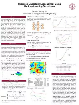
Abductive Networks at CAPS • Modeling/forecasting electric energy consumption • Modeling/forecasting meteorological data • Modeling of petrochemical processes • Oil and gas reservoir characterization • Medical diagnostics • Identification/Determination of radioisotopes and peak fitting in nuclear spectroscopy • Online monitoring of vibrations on vacuum pumps. • Direct estimation of noisy sinusoids
Proposed Work Apply abductive networks data-based modeling to the important areas of: • Electrical load modeling and forecasting at power utilities of the kingdom. • Hourly air temperature forecasts that may be required.
Benefits to Client • Transparent and accurate forecasters for economic and reliable operation • Comparison with existing models • Improve understanding of daily, weakly, and seasonal load variations • Determine social, economic, and weather factors influencing load • Introduce the use of modern computational intelligence techniques • Train junior engineers in load forecasting
Outline of Work 1. Identify application area 2. Determine relevant input variables 3. Select data sets for model development 4. Data preprocessing: Scan for outliers and missing data, trend adjustment, normalization, transformations, … 5. Model development 6. Model evaluation and analysis 7. Model integration into client setup 8. Assess performance, compare with present practices.
Examples of relevant modeling and forecasting applications at CAPS • Monthly electrical energy consumption in the Eastern Province • Daily maximum temperatures at Dhahran • Hourly electrical load forecasting using data from the USA
Modeling the Monthly Electrical Energy Consumption in the Eastern Province • Domestic Electrical Energy Consumption was modeled in terms of six exogenous parameters • 6-year data: (5 years for training, 1 year forecasted for evaluation) • Derived analytical model relationships from simplified models
Monthly Electrical Energy Consumption:The data set • Six Inputs: • Month Index (m): m=1,2,…,72 • Monthly average of the global solar radiation (S) • Population (P) • Gross domestic product per capita (G) • Monthly average of the daily mean air temperature (T) • Monthly average of the daily mean relative humidity (H) • One Output: • Monthly Domestic Electrical Energy Consumption(E)
S P G Monthly Electrical Energy Consumption: The Model Automatically selects the most relevant inputs as: m, H, and T Ignores remaining inputs Gives an overall analytical model relationship
Training Evaluation Aug 1987 Monthly Electrical Energy Consumption:Model Performance MAPE Error over Evaluation year: 5.6% Previous regression model gave MAPE = 9.2%.
Modeling the Maximum Daily Air Temperature (TX) • TX was modeled in terms of average temperatures (TA) for the previous three days: TX (d+1) = F [TA (d-2), TA (d-1), TA (d)] • 1987 year data for training, 1988 data for evaluation. • Derived analytical model relationships.
Maximum Daily Air Temperature (TX): The Model TX(d+1) = 5.243 + 0.272 TA (d-2) – 0.589 TA (d-1) + 1.339 TA (d)
Maximum Daily Air Temperature (TX):Model Performance Evaluation on 1988 data: MAE = 2.1 °C
Hourly electrical load forecasting Using Abductive Networks • Hourly load and temperature data for 6 years (1985-1990) from Puget Power, Seattle, USA* • 5-year data (1985-89) for model training and 1990 data for evaluation. • Developed 24 dedicated models that forecast tomorrow’s hourly load curve for any day of the year. ______________________________________________ * Courtesy Professor M. A. El-Sharkawi, University of Washington, Seattle, USA.
The Data Set Available Data: • 24 daily hourly loads (L1,L2,…,L24), MW • 24 daily hourly temperatures (T1,T2,…,T24), °F Generated Data: • Tmax and Tmin from hourly temperatures • Used actual Tmax and Tmin for next day as forecasted valuesETmax and ETmin. • Classified the forecasted day as: Working day, Saturday, Sunday, or Holiday. Represented as 4 binary inputs.
Average Annual Upward Trend: 3.6% Evaluation:364 Records 1985 Training: 1821 Records 1989 1990 Trend Removed by normalizing to 1989 mean
2 Hourly Load Forecasters 24 Load Forecaster for Hour h 24 off L(i), Hourly Loads on day (d-1) Load Forecaster for Hour h 2 Tmin, Tmax on day (d-1) 1 Tmine, Tmaxe Estimated for day d Le(d,h) Forecasted Load at hour h, day d 4 Day type code for day d Total : 32 inputs
Examples of Hourly Load Forecasters:Hour 1 (Midnight) Model Structure: Out of the 32 inputs, only 3 load inputs are selected No temperature inputs No day-type inputs 1-layer nonlinear model X1 = -4.52 + 0.00303 L3 X2 = -4.66 + 0.00295 L20 X3 = -5.61 + 0.00315 L24 Y = 0.125 X1 + 0.868 X3 – 0.115 X1 X2 + 0.0506 X1 X3 + 0.0582 X2 X3 LE1 = 1600 + 312 Y
Hour 1 (Midnight) Model Performance:
Examples of Hourly Load Forecasters:Hour 12 (Midday) Model Structure: More complex, 4-layers Only 4 load inputs, including same hour on previous day Only Sunday day-type input Forecasted temperature inputs
Hour 12 (Midday) Model Performance:
Forecasting Error Statistics Over the 1990 Evaluation Year: Overall MAPE = 2.67 %, with the following distribution: Overall MPE = - 0.16 %, mainly due to error in estimating growth for the forecasting year
Conclusions • Apply abductive networks machine learning to load modeling and forecasting. • Many advantages over neural networks, e.g. faster modeling and better explanations. • CAPS have used the technique in many areas, including energy, load, and meteorological forecasting. • Benefits include greater forecasting accuracy (reduced operating cost, improved security) and better insight into the load function.