Download
1 / 52
530 likes | 680 Views
Chapter 18: Data Analysis and Mining. Decision Support Systems Data Analysis and OLAP Data Warehousing Data Mining. Chapter 18: Data Analysis and Mining. Decision-support systems are used to make business decisions, often based on data collected by on-line transaction-processing systems.

E N D
Decision Support Systems Data Analysis and OLAP Data Warehousing Data Mining Chapter 18: Data Analysis and Mining
Decision-support systems are used to make business decisions, often based on data collected by on-line transaction-processing systems. Examples of business decisions: What items to stock? What insurance premium to change? To whom to send advertisements? Examples of data used for making decisions Retail sales transaction details Customer profiles (income, age, gender, etc.) Decision Support Systems
Data analysis tasks are simplified by specialized tools and SQL extensions Example tasks For each product category and each region, what were the total sales in the last quarter and how do they compare with the same quarter last year As above, for each product category and each customer category Statistical analysis packages (e.g., : S++) can be interfaced with databases Statistical analysis is a large field, but not covered here Data mining seeks to discover knowledge automatically in the form of statistical rules and patterns from large databases. A data warehouse archives information gathered from multiple sources, and stores it under a unified schema, at a single site. Important for large businesses that generate data from multiple divisions, possibly at multiple sites Data may also be purchased externally Decision-Support Systems: Overview
Online Analytical Processing (OLAP) Interactive analysis of data, allowing data to be summarized and viewed in different ways in an online fashion (with negligible delay) Data that can be modeled as dimension attributes and measure attributes are called multidimensional data. Measure attributes measure some value can be aggregated upon e.g. the attribute number of the sales relation Dimension attributes define the dimensions on which measure attributes (or aggregates thereof) are viewed e.g. the attributes item_name, color, and size of the sales relation Data Analysis and OLAP
The table above is an example of a cross-tabulation (cross-tab), also referred to as a pivot-table. Values for one of the dimension attributes form the row headers Values for another dimension attribute form the column headers Other dimension attributes are listed on top Values in individual cells are (aggregates of) the values of the dimension attributes that specify the cell. Cross Tabulation of sales by item-name and color
Relational Representation of Cross-tabs • Cross-tabs can be represented as relations • We use the value all is used to represent aggregates • The SQL:1999 standard actually uses null values in place of all despite confusion with regular null values
Data Cube • A data cube is a multidimensional generalization of a cross-tab • Can have n dimensions; we show 3 below • Cross-tabs can be used as views on a data cube
Pivoting: changing the dimensions used in a cross-tab is called Slicing: creating a cross-tab for fixed values only Sometimes called dicing, particularly when values for multiple dimensions are fixed. Rollup: moving from finer-granularity data to a coarser granularity Drill down: The opposite operation - that of moving from coarser-granularity data to finer-granularity data Online Analytical Processing
Hierarchies on Dimensions • Hierarchy on dimension attributes: lets dimensions to be viewed at different levels of detail • E.g. the dimension DateTime can be used to aggregate by hour of day, date, day of week, month, quarter or year
Cross Tabulation With Hierarchy • Cross-tabs can be easily extended to deal with hierarchies • Can drill down or roll up on a hierarchy
The earliest OLAP systems used multidimensional arrays in memory to store data cubes, and are referred to as multidimensional OLAP (MOLAP) systems. OLAP implementations using only relational database features are called relational OLAP (ROLAP) systems Hybrid systems, which store some summaries in memory and store the base data and other summaries in a relational database, are called hybrid OLAP (HOLAP)systems. OLAP Implementation
OLAP Implementation (Cont.) • Early OLAP systems precomputed all possible aggregates in order to provide online response • Space and time requirements for doing so can be very high • 2n combinations of group by • It suffices to precompute some aggregates, and compute others on demand from one of the precomputed aggregates • Can compute aggregate on (item-name, color) from an aggregate on (item-name, color, size) • For all but a few “non-decomposable” aggregates such as median • is cheaper than computing it from scratch • Several optimizations available for computing multiple aggregates • Can compute aggregate on (item-name, color) from an aggregate on (item-name, color, size) • Can compute aggregates on (item-name, color, size), (item-name, color) and (item-name) using a single sorting of the base data
The cube operation computes union of group by’s on every subset of the specified attributes E.g. consider the query select item-name, color, size, sum(number)fromsalesgroup by cube(item-name, color, size) This computes the union of eight different groupings of the sales relation: { (item-name, color, size), (item-name, color), (item-name, size), (color, size), (item-name), (color), (size), ( ) } where ( ) denotes an empty group by list. For each grouping, the result contains the null value for attributes not present in the grouping. Extended Aggregation in SQL:1999
Extended Aggregation (Cont.) • Relational representation of cross-tab that we saw earlier, but with null in place of all, can be computed by select item-name, color, sum(number)from salesgroup by cube(item-name, color) • The function grouping() can be applied on an attribute • Returns 1 if the value is a null value representing all, and returns 0 in all other cases. select item-name, color, size, sum(number),grouping(item-name) as item-name-flag,grouping(color) as color-flag,grouping(size) as size-flag,from salesgroup by cube(item-name, color, size) • Can use the function decode() in the select clause to replace such nulls by a value such as all • E.g. replace item-name in first query by decode( grouping(item-name), 1, ‘all’, item-name)
The rollup construct generates union on every prefix of specified list of attributes E.g. select item-name, color, size, sum(number)from salesgroup by rollup(item-name, color, size) Generates union of four groupings: { (item-name, color, size), (item-name, color), (item-name), ( ) } Rollup can be used to generate aggregates at multiple levels of ahierarchy. E.g., suppose table itemcategory(item-name, category) gives the category of each item. Then select category, item-name, sum(number)from sales, itemcategorywhere sales.item-name = itemcategory.item-namegroup by rollup(category, item-name) would give a hierarchical summary by item-name and by category. Extended Aggregation (Cont.)
Multiple rollups and cubes can be used in a single group by clause Each generates set of group by lists, cross product of sets gives overall set of group by lists E.g., select item-name, color, size, sum(number)from salesgroup by rollup(item-name), rollup(color, size) generates the groupings {item-name, ()} X {(color, size), (color), ()} = { (item-name, color, size), (item-name, color), (item-name), (color, size), (color), ( ) } Extended Aggregation (Cont.)
Ranking is done in conjunction with an order by specification. Given a relation student-marks(student-id, marks) find the rank of each student. select student-id, rank( ) over (order by marksdesc) as s-rankfrom student-marks An extra order by clause is needed to get them in sorted order select student-id, rank ( ) over (order by marksdesc) as s-rankfrom student-marks order by s-rank Ranking may leave gaps: e.g. if 2 students have the same top mark, both have rank 1, and the next rank is 3 dense_rank does not leave gaps, so next dense rank would be 2 Ranking
Ranking (Cont.) • Ranking can be done within partition of the data. • “Find the rank of students within each section.” select student-id, section,rank ( ) over (partition by section order by marks desc) as sec-rankfrom student-marks, student-sectionwhere student-marks.student-id = student-section.student-idorder by section, sec-rank • Multiple rank clauses can occur in a single select clause • Ranking is done after applying group by clause/aggregation
Ranking (Cont.) • Other ranking functions: • percent_rank (within partition, if partitioning is done) • cume_dist (cumulative distribution) • fraction of tuples with preceding values • row_number (non-deterministic in presence of duplicates) • SQL:1999 permits the user to specify nulls first or nulls last select student-id, rank ( ) over (order by marks desc nulls last) as s-rankfrom student-marks
For a given constant n, the ranking the function ntile(n) takes the tuples in each partition in the specified order, and divides them into n buckets with equal numbers of tuples. E.g.: select threetile, sum(salary)from (select salary, ntile(3) over (order by salary) as threetilefrom employee) as sgroup by threetile Ranking (Cont.)
Used to smooth out random variations. E.g.: moving average: “Given sales values for each date, calculate for each date the average of the sales on that day, the previous day, and the next day” Window specification in SQL: Given relation sales(date, value) select date, sum(value) over (order by date between rows 1 preceding and 1 following)from sales Examples of other window specifications: between rows unbounded preceding and current rows unbounded preceding range between 10 preceding and current row All rows with values between current row value –10 to current value range interval 10 day preceding Not including current row Windowing
Windowing (Cont.) • Can do windowing within partitions • E.g. Given a relation transaction (account-number, date-time, value), where value is positive for a deposit and negative for a withdrawal • “Find total balance of each account after each transaction on the account” select account-number, date-time,sum (value ) over (partition by account-number order by date-timerows unbounded preceding)as balancefrom transactionorder by account-number, date-time
Data Warehousing • Data sources often store only current data, not historical data • Corporate decision making requires a unified view of all organizational data, including historical data • A data warehouse is a repository (archive) of information gathered from multiple sources, stored under a unified schema, at a single site • Greatly simplifies querying, permits study of historical trends • Shifts decision support query load away from transaction processing systems
When and how to gather data Source driven architecture: data sources transmit new information to warehouse, either continuously or periodically (e.g. at night) Destination driven architecture: warehouse periodically requests new information from data sources Keeping warehouse exactly synchronized with data sources (e.g. using two-phase commit) is too expensive Usually OK to have slightly out-of-date data at warehouse Data/updates are periodically downloaded form online transaction processing (OLTP) systems. What schema to use Schema integration Design Issues
More Warehouse Design Issues • Data cleansing • E.g. correct mistakes in addresses (misspellings, zip code errors) • Merge address lists from different sources and purge duplicates • How to propagate updates • Warehouse schema may be a (materialized) view of schema from data sources • What data to summarize • Raw data may be too large to store on-line • Aggregate values (totals/subtotals) often suffice • Queries on raw data can often be transformed by query optimizer to use aggregate values
Warehouse Schemas • Dimension values are usually encoded using small integers and mapped to full values via dimension tables • Resultant schema is called a star schema • More complicated schema structures • Snowflake schema: multiple levels of dimension tables • Constellation: multiple fact tables
Data Mining • Data mining is the process of semi-automatically analyzing large databases to find useful patterns • Prediction based on past history • Predict if a credit card applicant poses a good credit risk, based on some attributes (income, job type, age, ..) and past history • Predict if a pattern of phone calling card usage is likely to be fraudulent • Some examples of prediction mechanisms: • Classification • Given a new item whose class is unknown, predict to which class it belongs • Regression formulae • Given a set of mappings for an unknown function, predict the function result for a new parameter value
Data Mining (Cont.) • Descriptive Patterns • Associations • Find books that are often bought by “similar” customers. If a new such customer buys one such book, suggest the others too. • Associations may be used as a first step in detecting causation • E.g. association between exposure to chemical X and cancer, • Clusters • E.g. typhoid cases were clustered in an area surrounding a contaminated well • Detection of clusters remains important in detecting epidemics
Classification rules help assign new objects to classes. E.g., given a new automobile insurance applicant, should he or she be classified as low risk, medium risk or high risk? Classification rules for above example could use a variety of data, such as educational level, salary, age, etc. person P, P.degree = masters and P.income > 75,000 P.credit = excellent person P, P.degree = bachelors and (P.income 25,000 and P.income 75,000) P.credit = good Rules are not necessarily exact: there may be some misclassifications Classification rules can be shown compactly as a decision tree. Classification Rules
Training set: a data sample in which the classification is already known. Greedy top down generation of decision trees. Each internal node of the tree partitions the data into groups based on a partitioning attribute, and a partitioning condition for the node Leaf node: all (or most) of the items at the node belong to the same class, or all attributes have been considered, and no further partitioning is possible. Construction of Decision Trees
Pick best attributes and conditions on which to partition The purity of a set S of training instances can be measured quantitatively in several ways. Notation: number of classes = k, number of instances = |S|, fraction of instances in class i = pi. The Gini measure of purity is defined as [ Gini (S) = 1 - When all instances are in a single class, the Gini value is 0 It reaches its maximum (of 1 –1 /k) if each class the same number of instances. k p2i i- 1 Best Splits
r |Si| |S| purity (Si) pilog2 pi k i= 1 i- 1 Best Splits (Cont.) • Another measure of purity is the entropy measure, which is defined as entropy (S) = – • When a set S is split into multiple sets Si, I=1, 2, …, r, we can measure the purity of the resultant set of sets as: purity(S1, S2, ….., Sr) = • The information gain due to particular split of S into Si, i = 1, 2, …., r Information-gain (S, {S1, S2, …., Sr) = purity(S ) – purity (S1, S2, … Sr)
Measure of “cost” of a split: Information-content (S, {S1, S2, ….., Sr})) = – Information-gain ratio = Information-gain (S, {S1, S2, ……, Sr}) Information-content (S, {S1, S2, ….., Sr}) The best split is the one that gives the maximum information gain ratio r |Si| |S| |Si| |S| log2 i- 1 Best Splits (Cont.)
Finding Best Splits • Categorical attributes (with no meaningful order): • Multi-way split, one child for each value • Binary split: try all possible breakup of values into two sets, and pick the best • Continuous-valued attributes (can be sorted in a meaningful order) • Binary split: • Sort values, try each as a split point • E.g. if values are 1, 10, 15, 25, split at 1, 10, 15 • Pick the value that gives best split • Multi-way split: • A series of binary splits on the same attribute has roughly equivalent effect
Procedure GrowTree (S )Partition (S );Procedure Partition (S)if ( purity (S ) > p or |S| < s ) thenreturn;for each attribute A evaluate splits on attribute A; Use best split found (across all attributes) to partitionS into S1, S2, …., Sr,for i = 1, 2, ….., r Partition (Si ); Decision-Tree Construction Algorithm
Other Types of Classifiers • Neural net classifiers are studied in artificial intelligence and are not covered here • Bayesian classifiers use Bayes theorem, which says p (cj | d ) = p (d | cj ) p (cj ) p ( d )where p (cj | d ) = probability of instance d being in class cj, p (d | cj ) = probability of generating instance d given class cj, p (cj)= probability of occurrence of class cj, and p (d ) = probability of instance d occuring
Naïve Bayesian Classifiers • Bayesian classifiers require • computation of p (d | cj ) • precomputation of p (cj ) • p (d ) can be ignored since it is the same for all classes • To simplify the task, naïve Bayesian classifiers assume attributes have independent distributions, and thereby estimate p (d | cj) = p (d1 | cj ) * p (d2 | cj ) * ….* (p (dn | cj ) • Each of the p (di | cj ) can be estimated from a histogram on di values for each class cj • the histogram is computed from the training instances • Histograms on multiple attributes are more expensive to compute and store
Regression deals with the prediction of a value, rather than a class. Given values for a set of variables, X1, X2, …, Xn, we wish to predict the value of a variable Y. One way is to infer coefficients a0, a1, a1, …, an such thatY = a0 + a1 * X1 + a2 * X2 + … + an * Xn Finding such a linear polynomial is called linear regression. In general, the process of finding a curve that fits the data is also called curve fitting. The fit may only be approximate because of noise in the data, or because the relationship is not exactly a polynomial Regression aims to find coefficients that give the best possible fit. Regression
Retail shops are often interested in associations between different items that people buy. Someone who buys bread is quite likely also to buy milk A person who bought the book Database System Concepts is quite likely also to buy the book Operating System Concepts. Associations information can be used in several ways. E.g. when a customer buys a particular book, an online shop may suggest associated books. Association rules: bread milk DB-Concepts, OS-Concepts Networks Left hand side: antecedent, right hand side: consequent An association rule must have an associated population; the population consists of a set of instances E.g. each transaction (sale) at a shop is an instance, and the set of all transactions is the population Association Rules
Rules have an associated support, as well as an associated confidence. Supportis a measure of what fraction of the population satisfies both the antecedent and the consequent of the rule. E.g. suppose only 0.001 percent of all purchases include milk and screwdrivers. The support for the rule is milk screwdrivers is low. Confidenceis a measure of how often the consequent is true when the antecedent is true. E.g. the rule bread milk has a confidence of 80 percent if 80 percent of the purchases that include bread also include milk. Association Rules (Cont.)
We are generally only interested in association rules with reasonably high support (e.g. support of 2% or greater) Naïve algorithm Consider all possible sets of relevant items. For each set find its support (i.e. count how many transactions purchase all items in the set). Large itemsets: sets with sufficiently high support Use large itemsets to generate association rules. From itemset A generate the rule A - {b } b for each b A. Support of rule = support (A). Confidence of rule = support (A ) / support (A - {b }) Finding Association Rules
Determine support of itemsets via a single pass on set of transactions Large itemsets: sets with a high count at the end of the pass If memory not enough to hold all counts for all itemsets use multiple passes, considering only some itemsets in each pass. Optimization: Once an itemset is eliminated because its count (support) is too small none of its supersets needs to be considered. The a priori technique to find large itemsets: Pass 1: count support of all sets with just 1 item. Eliminate those items with low support Pass i: candidates: every set of i items such that all its i-1 item subsets are large Count support of all candidates Stop if there are no candidates Finding Support
Other Types of Associations • Basic association rules have several limitations • Deviations from the expected probability are more interesting • E.g. if many people purchase bread, and many people purchase cereal, quite a few would be expected to purchase both • We are interested in positive as well as negative correlations between sets of items • Positive correlation: co-occurrence is higher than predicted • Negative correlation: co-occurrence is lower than predicted • Sequence associations / correlations • E.g. whenever bonds go up, stock prices go down in 2 days • Deviations from temporal patterns • E.g. deviation from a steady growth • E.g. sales of winter wear go down in summer • Not surprising, part of a known pattern. • Look for deviation from value predicted using past patterns
Clustering • Clustering: Intuitively, finding clusters of points in the given data such that similar points lie in the same cluster • Can be formalized using distance metrics in several ways • Group points into k sets (for a given k) such that the average distance of points from the centroid of their assigned group is minimized • Centroid: point defined by taking average of coordinates in each dimension. • Another metric: minimize average distance between every pair of points in a cluster • Has been studied extensively in statistics, but on small data sets • Data mining systems aim at clustering techniques that can handle very large data sets • E.g. the Birch clustering algorithm (more shortly)
Hierarchical Clustering • Example from biological classification • (the word classification here does not mean a prediction mechanism) chordata mammalia reptilialeopards humans snakes crocodiles • Other examples: Internet directory systems (e.g. Yahoo, more on this later) • Agglomerative clustering algorithms • Build small clusters, then cluster small clusters into bigger clusters, and so on • Divisive clustering algorithms • Start with all items in a single cluster, repeatedly refine (break) clusters into smaller ones
Clustering Algorithms • Clustering algorithms have been designed to handle very large datasets • E.g. the Birch algorithm • Main idea: use an in-memory R-tree to store points that are being clustered • Insert points one at a time into the R-tree, merging a new point with an existing cluster if is less than some distance away • If there are more leaf nodes than fit in memory, merge existing clusters that are close to each other • At the end of first pass we get a large number of clusters at the leaves of the R-tree • Merge clusters to reduce the number of clusters