Download
1 / 29
300 likes | 343 Views
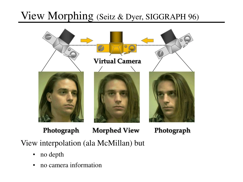
Virtual Camera. Photograph. Photograph. Morphed View. View Morphing (Seitz & Dyer, SIGGRAPH 96). View interpolation (ala McMillan) but no depth no camera information. But First: Multi-View Projective Geometry. Last time (single view geometry) Vanishing Points Points at Infinity

E N D
Virtual Camera Photograph Photograph Morphed View View Morphing (Seitz & Dyer, SIGGRAPH 96) • View interpolation (ala McMillan) but • no depth • no camera information
But First: Multi-View Projective Geometry • Last time (single view geometry) • Vanishing Points • Points at Infinity • Vanishing Lines • The Cross-Ratio • Today (multi-view geometry) • Point-line duality • Epipolar geometry • The Fundamental Matrix • All quantities on these slides are in homogeneous coordinates except when specified otherwise
(x,y,1) Cartesian plane The Projective Plane • Why do we need homogeneous coordinates? • represent points at infinity, homographies, perspective projection, multi-view relationships • What is the geometric intuition? • The projective plane f (fx,fy,f) image plane (projective) (0,0,0) focal point • Each point(x,y) on the plane is represented by a rays(x,y,1) • Cartesian coordinates (x,y,z)(x/z, y/z)
Projective Lines • A point is a ray in projective space • How would we represent a line? image plane • A line is a plane of rays • all rays (x,y,z) satisfying: ax + by + cz = 0 • A line is also represented as a homogeneous 3-vector l
l1 p l l2 Point and Line Duality • A line l is a homogeneous 3-vector (a ray) • It is to every point (ray) p on the line: lTp=0 p2 p1 • What is the line l spanned by points p1 and p2 ? • l is to p1 and p2 l = p1p2 • l is the plane normal • What is the intersection of two lines l1 and l2 ? • p is to l1 and l2 p = l1l2 • Points and lines are dual in projective space • every property of points also applies to lines (e.g., cross-ratio)
Homographies of Points and Lines • We’ve seen lots of names for these • Planar perspective transformations • Homographies • Texture-mapping transformations • Collineations • Computed by 3x3 matrix multiplication • To transform a point: p’ = Hp • To transform a line: lTp=0 l’Tp’=0 • 0 = lTp = lTH-1Hp = lTH-1p’ l’T = lTH-1 • lines are transformed by(H-1)T
3D Projective Geometry • These concepts generalize naturally to 3D • Homogeneous coordinates • Projective 3D points have four coords: X = (X,Y,Z,W) • Duality • A plane is also represented by a 4-vector • Points and planes are dual in 3D: TP=0 • Projective transformations • Represented by 4x4 matrices T: P’ = TP, ’ = (T-1)T • Cross-ratio of planes • However • Can’t use cross-products in 4D. We need new tools • Grassman-Cayley Algebra • generalization of cross product, allows interactions between points, lines, and planes via “meet” and “join” operators • Won’t get into this stuff today
It’s useful to decompose into T R project A Then we can write the projection as: 3D to 2D: Perspective Projection • Matrix Projection:
scene point image plane focal point Multi-View Projective Geometry • How to relate point positions in different views? • Central question in image-based rendering • Projective geometry gives us some powerful tools • constraints between two or more images • equations to transfer points from one image to another
epipolar plane epipolar line epipolar line epipoles Epipolar Geometry • What does one view tell us about another? • Point positions in 2nd view must lie along a known line • Epipolar Constraint • Extremely useful for stereo matching • Reduces problem to 1D search along conjugateepipolar lines • Also useful for view interpolation...
Transfer from Epipolar Lines • What does one view tell us about another? • Point positions in 2nd view must lie along a known line output image input image input image • Two views determines point position in a third image • But doesn’t work if point is in the trifocal plane spanned by all three cameras • bad case: three cameras are colinear
p Y Y p’ X T Z Z X R Epipolar Algebra • How do we compute epipolar lines? • Can trace out lines, reproject. But that is overkill p’ = Rp + T • Note that p’ is toTp’ • So 0 = p’T Tp = p’T T(Rp + T) = p’T T(Rp)
Therefore: • Where E =TR is the 3x3 “essential matrix” • Holds whenever p and p’ correspond to the same scene point Simplifying: p’T T(Rp) = 0 • We can write a cross-product ab as a matrix equation • a b = Ab where • Properties of E • Ep is the epipolar line of p; p’T E is the epipolar line of p’ • p’T E p = 0 for every pair of corresponding points • 0 = Ee = e’T E where e and e’ are the epipoles • E has rank < 3, has 5 independent parameters • E tells us everything about the epipolar geometry
Linear Multiview Relations • The Essential Matrix: 0 = p’T E p • First derived by Longuet-Higgins, Nature 1981 • also showed how to compute camera R and T matrices from E • E has only 5 free parameters (three rotation angles, two transl. directions) • Only applies when cameras have same internal parameters • same focal length, aspect ratio, and image center • The Fundamental Matrix: 0 = p’T F p • F = (A’-1)T E A-1, where A3x3 and A’3x3 contain the internal parameters • Gives epipoles, epipolar lines • F (like E) is defined only up to a scale factor and has rank 2 (7 free params) • Generalization of the essential matrix • Can’t uniquely solve for R and T (or A and A’) from F • Can be computed using linear methods • R. Hartley, In Defence of the 8-point Algorithm, ICCV 95 • Or nonlinear methods • Xu & Zhang, Epipolar Geometry in Stereo, Motion and Object Recognition, 1996
The Trifocal Tensor • What if you have three views? • Can compute 3 pairwise fundamental matrices • However there are more constraints • it should be possible to resolve the trifocal problem • Answer: the trifocal tensor • introduced by Shashua, Hartley in 1994/1995 • a 3x3x3 matrix T (27 parameters) • gives all constraints between 3 views • can use to generate new views without trifocal probs. [Shai & Avidan] • linearly computable from point correspondences • How about four views? five views? N views? • There is a quadrifocal tensor [Faugeras & Morrain, Triggs, 1995] • But: all the constraints are expressed in the trifocal tensors, obtained by considering every subset of 3 cameras
Virtual Camera Photograph Photograph Morphed View View Morphing (Seitz & Dyer, SIGGRAPH 96) • View interpolation (ala McMillan) but • no depth • no camera information
Uniqueness Result • Given • Any two images of a Lambertian scene • No occlusions • Result: all views along C1C2 are uniquely determined • View Synthesis is solvable when • Cameras are uncalibrated • Dense pixel correspondence is not available • Shape reconstruction is impossible
Uniqueness Result • Relies on Monotonicity Assumption • Left-to-right ordering of points is the same in both images • used often to facilitate stereo matching • Implies no occlusions on line between C1 and C2
Image Morphing Photograph Photograph Photograph Morphed Image Photograph • Linear Interpolation of 2D shape and color
Image Morphing for View Synthesis? • We want to high quality view interpolations • Can image morphing do this? • Goal: extend to handle changes in viewpoint • Produce valid camera transitions
Special Case: Parallel Cameras LeftImage MorphedImage RightImage • Morphing parallel views new parallel views • Projection matrices have a special form • third rows of projection matrices are equal • Linear image motion linear camera motion
Uncalibrated Prewarping • Parallel cameras have a special epipolar geometry • Epipolar lines are horizontal • Corresponding points have the same y coordinate in both images • What fundamental matrix does this correspond to? • Prewarp procedure: • Compute F matrix given 8 or more correspondences • Compute homographies H and H’ such that • each homography composes two rotations, a scale, and a translation • Transform first image by H-1, second image by H’-1
1. Prewarp • align views • 2. Morph • move camera
1. Prewarp • align views
1. Prewarp • align views • 2. Morph • move camera
1. Prewarp • align views • 2. Morph • move camera • 3. Postwarp • point camera
Corrected Photographs Face Recognition
View Morphing Summary • Additional Features • Automatic correspondence • N-view morphing • Real-time implementation • Pros • Don’t need camera positions • Don’t need shape/Z • Don’t need dense correspondence • Cons • Limited to interpolation (although not with three views) • Problems with occlusions (leads to ghosting) • Prewarp can be unstable (need good F-estimator)
Some Applications of Projective Geometry • Homogeneous coordinates in computer graphics • Metrology • Single view • Multi-view • Stereo correspondence • View interpolation and transformation • Camera calibration • Invariants • Object recognition • Pose estimation • Others...