Download

1 / 39
390 likes | 547 Views
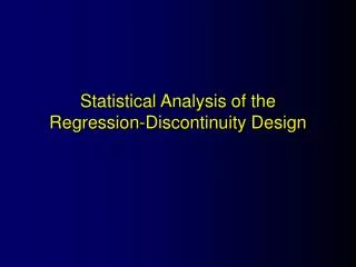
Statistical Analysis of the Nonequivalent Groups Design. Analysis Requirements. N O X O N O O. Pre-post Two-group Treatment-control (dummy-code). Analysis of Covariance. y i = 0 + 1 X i + 2 Z i + e i. y i = outcome score for the i th unit

E N D
Analysis Requirements N O X O N O O • Pre-post • Two-group • Treatment-control (dummy-code)
Analysis of Covariance yi = 0 + 1Xi + 2Zi + ei yi = outcome score for the ith unit 0 = coefficient for the intercept 1 = pretest coefficient 2 = mean difference for treatment Xi = covariate Zi = dummy variable for treatment(0 = control, 1= treatment) ei = residual for the ith unit where:
9 0 8 0 7 0 t s e t 6 0 t s o p 5 0 4 0 3 0 3 0 4 0 5 0 6 0 7 0 8 0 p r e t e s t The Bivariate Distribution Program group scores 15-points higher on Posttest. Program group has a 5-point pretest Advantage.
Regression Results yi = 18.7 + .626Xi + 11.3Zi • Result is biased! • CI.95(2=10) = 2±2SE(2) = 11.2818±2(.5682) = 11.2818±1.1364 • CI = 10.1454 to 12.4182 Predictor Coef StErr t p Constant 18.714 1.969 9.50 0.000 pretest 0.62600 0.03864 16.20 0.000 Group 11.2818 0.5682 19.85 0.000
9 0 8 0 7 0 t s e t 6 0 t s o p 5 0 4 0 3 0 3 0 4 0 5 0 6 0 7 0 8 0 p r e t e s t The Bivariate Distribution Regression line slopes are biased. Why?
Y X Regression and Error No measurement error
Y X Y X Regression and Error No measurement error Measurement error on the posttest only
Y X Y X Y X Regression and Error No measurement error Measurement error on the posttest only Measurement error on the pretest only
How Regression Fits Lines Method of least squares
How Regression Fits Lines Method of least squares Minimize the sum of the squares of the residuals from the regression line.
Y X How Regression Fits Lines Method of least squares Minimize the sum of the squares of the residuals from the regression line. Least squares minimizes on y not x.
Y X How Error Affects Slope No measurement error, No effect
Y X Y X How Error Affects Slope No measurement error, no effect. Measurement error on the posttest only, adds variability around regression line, but doesn’t affect the slope
Y X Y X Y X How Error Affects Slope No measurement error, no effect. Measurement error on the posttest only, adds variability around regression line, but doesn’t affect the slope. Measurement error on the pretest only: Affects slope Flattens regression lines
Y X Y X Y Y X X How Error Affects Slope Measurement error on the pretest only: Affects slope Flattens regression lines
Y X Y X Y Y X X How Error Affects Slope Notice that the true result in all three cases should be a null (no effect) one.
Y X How Error Affects Slope Notice that the true result in all three cases should be a null (no effect) one. Null case
Y X How Error Affects Slope But with measurement error on the pretest, we get a pseudo-effect. Pseudo-effect
Where Does This Leave Us? • Traditional ANCOVA looks like it should work on NEGD, but it’s biased. • The bias results from the effect of pretest measurement errorunder the least squares criterion. • Slopes are flattened or “attenuated”.
What’s the Answer? • If it’s a pretest problem, let’s fix the pretest. • If we could remove the errorfrom the pretest, it would fix the problem. • Can we adjust pretest scoresfor error? • What do we know about error?
What’s the Answer? • We know that if we had no error, reliability = 1; all error, reliability=0. • Reliability estimates the proportion of true score. • Unreliability=1-Reliability. • This is the proportion of error! • Use this to adjust pretest.
What Would a Pretest Adjustment Look Like? Original pretest distribution
What Would a Pretest Adjustment Look Like? Original pretest distribution Adjusted dretest distribution
Y X How Would It Affect Regression? The regression The pretest distribution
Y X How Would It Affect Regression? The regression The pretest distribution
Y X How Far Do We Squeeze the Pretest? • Squeeze inward an amount proportionate to the error. • If reliability=.8, we want to squeeze in about 20% (i.e., 1-.8). • Or, we want pretest to retain 80%of it’s original width.
Adjusting the Pretest for Unreliability _ _ Xadj = X + r(X - X)
Adjusting the Pretest for Unreliability _ _ Xadj = X + r(X - X) where:
Adjusting the Pretest for Unreliability _ _ Xadj = X + r(X - X) where: Xadj = adjusted pretest value
Adjusting the Pretest for Unreliability _ _ Xadj = X + r(X - X) where: Xadj = adjusted pretest value _ X = original pretest value
Adjusting the Pretest for Unreliability _ _ Xadj = X + r(X - X) where: Xadj = adjusted pretest value _ X = original pretest value r = reliability
Reliability-CorrectedAnalysis of Covariance yi = 0 + 1Xadj + 2Zi + ei yi = outcome score for the ith unit 0 = coefficient for the intercept 1 = pretest coefficient 2 = mean difference for treatment Xadj = covariate adjusted for unreliability Zi = dummy variable for treatment(0 = control, 1= treatment) ei = residual for the ith unit where:
Regression Results yi = -3.14 + 1.06Xadj + 9.30Zi • Result is unbiased! • CI.95(2=10) = 2±2SE(2) = 9.3048±2(.6166) = 9.3048±1.2332 • CI = 8.0716 to 10.5380 Predictor Coef StErr t p Constant -3.141 3.300 -0.95 0.342 adjpre 1.06316 0.06557 16.21 0.000 Group 9.3048 0.6166 15.09 0.000
pretest posttest pretest posttest MEAN MEAN STD DEV STD DEV Comp 49.991 50.008 6.985 7.549 Prog 54.513 64.121 7.037 7.381 ALL 52.252 57.064 7.360 10.272 Graph of Means
pretest adjpre posttest pretest adjpre posttest MEAN MEAN MEAN STD DEV STD DEV STD DEV Comp 49.991 49.991 50.008 6.985 3.904 7.549 Prog 54.513 54.513 64.121 7.037 4.344 7.381 ALL 52.252 52.252 57.064 7.360 4.706 10.272 Adjusted Pretest • Note that the adjusted means are the same as the unadjusted means. • The only thing that changes is the standard deviation (variability).
9 0 8 0 7 0 t s e t 6 0 t s o p 5 0 4 0 3 0 3 0 4 0 5 0 6 0 7 0 8 0 p r e t e s t Original Regression Results Pseudo-effect=11.28 Original
9 0 8 0 7 0 t s e t 6 0 t s o p 5 0 4 0 3 0 3 0 4 0 5 0 6 0 7 0 8 0 p r e t e s t Corrected Regression Results Pseudo-effect=11.28 Original Effect=9.31 Corrected