Download
1 / 59
590 likes | 592 Views
Data Mining Techniques for Query Relaxation. Query Relaxation via Abstraction. Abstraction must be automated for Large domains Unfamiliar domains. Abstraction is context dependent: 6’9” guard big guard 6’9” forward medium forward 6’9” center small center.

E N D
Query Relaxation via Abstraction • Abstraction must be automated for • Large domains • Unfamiliar domains Abstraction is context dependent: 6’9” guard big guard 6’9” forward medium forward 6’9” center small center Heights of guards A conceptual query: Find me a big guard < 6’ <= 6’4” > 6’4” small medium large
Related Work • Maximum Entropy (ME) method: • Maximization of entropy (- Sp log p) • Only considers frequency distribution • Conceptual clustering systems: • Only allows non-numerical values (COBWEB) • Assume a certain distribution (CLASSIT)
Supervised vs. Unsupervised Learning Supervised Learning: Given instances with known class information, generate rules/decision tree that can be used to infer class of future instances Examples: ID3, Statistical Pattern Recognition Unsupervised Learning: Given instances with unknownclass information, generate concept tree that cluster instances into similar classes Examples: COBWEB, TAH Generation (DISC, PBKI)
Automatic Construction of TAHs • Necessary for Scaling up CoBase • Sources of Knowledge • Database Instance • Attribute Value Distributions • Inter-Attribute Relationships • Query and Answer Statistics • Domain Expert • Approach • Generate Initial TAH • With Minimal Expert Effort • Edit the Hierarchy to Suit • Application Context • User Profile
For Clustering Attribute Instances with Non-Numerical Values
Pattern-Based Knowledge Induction (PKI) • Rule-Based • Cluster attribute values into TAH based on other attributes in the relation • Provides Attribute Correlation value
Definitions The cardinality of a pattern P, denoted |P|, is the number of distinct objects that match P. The confidence of a rule A B, denoted byx(A B), is x (A B) = |AIB| / |A| Let A B be a rule that applies to a relation R. The support of the rule over R is defined as h(A B) = |A| / |R|
Knowledge Inference: A Three-Step Process Step 1: Infer Rules Consider all rules of basic form A B. Calculate Confidence and Support. Confidence measures how well a rule applies to the database. A B has a confidence of .75 means that if A holds, B has a 75% chance of holding as well. Support measures how often a rule applies to the database. A B has a support of 10 means that it applies to 10 tuples in the database (A holds for 10 tuples).
Knowledge Inference (cont’d) Step 2: Combine Rules If two rules share a consequence and have the same attribute as a premise (with different values), then those values are candidates for clustering. Color = red style = “sport” (x1) Color = black style = “sport” (x2) Suggests red and black should be clustered. Correlation is product of the confidences of the two rules: g = x1 x x2
Clustering Algorithm: Binary Cluster (Greedy Algorithm) repeat INDUCE RULES and determine g sort g in descending order for each g(ai, aj) if ai and aj are unclustered replace ai and aj in DB with joint value Ji,j until fully clustered Approximate n-ary g using binary g cluster a set of n values if the g between all pairs is above threshold Decrease threshold and repeat
Knowledge Inference (cont’d) Step 3: Combine Correlations Clustering Correlation between two values is the weighted sum of their correlations. Combines all the evidence that two values should be clustered together into a single number (g(a1, a2)). g(a1, a2) = S i = 1wix x(A = a1 Bi = bi) x x(A = a2 Bi = bi) / (m-1) Where a1, a2 are values of attribute A, and there are m attributes B1, …, Bm in the relation with corresponding weights w1, …, wm m
Pattern-Based Knowledge Induction (Example) A B C a1 b1 c1 a1 b2 c1 a2 b1 c1 a3 b2 c1 1st iteration Rules: A = a1 B = b1 confidence = 0.5 A = a2 B = b1 confidence = 1.0 A = a1 C = c1 confidence = 1.0 A = a2 C = c1 confidence = 1.0 correlation (a1, a2) = 0.5x1.0+1.0x1.0/ 2 = 0.75 correlation (a1, a3) = 0.75 correlation (a2, a3) = 0.5
A = a12 B = b2 confidence = 0.33 A = a3 B = b2 confidence = 1.0 A = a12 C = c1 confidence = 1.0 A = a3 C = c1 confidence = 1.0 correlation (a12, a3) = = 0.67 0.33x1.0+1.0x1.0 2 Pattern-Based Knowledge Induction (cont’d) 2nd iteration 0.67 A B C a12 b1 c1 a12 b2 c1 a12 b1 c1 a3 b2 c1 0.75 a3 a1 a2
Example for Non-Numerical Attribute ValueThe PEOPLE Relation
Cor(a12, a3) is computed as follows: • Attribute origin: Same (Holland) contributes 1.0 • Attribute hair: Same contributes 1.0 • Attribute eye: Different contributes 0.0 • Attribute height: Overlap on MEDIUM • 5/10 of a12 and 2/2 of a3 contributes 5/10 * 2/2 = 0.5 cor(a12, a3) = 1/4 * (1+1+0+0.5) = 0.63
Correlation Computation Compute correlation between European and Asian. • Attributes ORIGIN and HAIR COLOR • No overlap between Europe and Asia, no contributions to correlation • Attribute EYE COLOR • BROWN is the only attribute that has overlap • 1 out of 24 Europeans have BROWN • 12 out of 12 Asians have BROWN • Attribute BROWN contributes 1/24 * 12/12 = 0.0416 • Attribute Height • SHORT: 5/24 Europeans and 8/12 of Asians • Medium: 11/24 and 3/12 • Tall: 8/24 and 1/12 • Attribute HEIGHT contributes 5/24 * 8/12 + 11/24 * 3/12 + 8/12 * 1/12 = 0.2812 Total Contribution = 0.0416 + 0.2812 = 0.3228 Correlation = 1/4(0.3228) = 0.0807
Extensions • Pre-clustering • For non-discrete domains • Reduces computational complexity • Expert Direction • Identify complex rules • Eliminate unrelated attributes • Eliminating Low-Popularity Rules • Set Popularity Threshold q • Do not keep rules below q • Saves Time and Space • Loses Knowledge about Uncommon Data In the Transportation Example, q = 2 improves efficiency by nearly 80%. Statistical sampling for very large domains.
Conventional Clustering Methods:I. Maximum Entropy (ME) Maximization of entropy (- Sp log p) Only considers frequency distribution: Example: {1,1,2,99,99,100} and {1,1,2,3,100,100} have the same entropy (2/6,1/6,2/6,1/6) ME cannot distinguish between (1) {1,1,2},{99,99,100}: good partition (2) {1,1,2},{3,100,100}: bad partition Me does not consider value distribution. Clusters have no semantic meaning.
Conventional Clustering Methods:II. Biggest Gap (BG) Consider only value distribution Find cuts at biggest gaps {1,1,1,10,10,20} is partitioned to {1,1,1,10,10} and {20} bad A good partition: {1,1,1} and {10,10,20}
A 10+1+2 = 3 ( ) 3 3 = 9 B C 11+0+1 = 2 ( ) 3 3 = 9 12+1+0 = 3 ( ) 1 2 3 4 5 3 3 = 9 Distribution Sensitive Clustering (DISC) Example
Relaxation Error: RE(B) = average pair-wise difference = 3 + 2 + 3 = 8 9 9 9 9 RE(C) = 0.5 RE(A) = 2.08 correlation (B) = 1 - RE(B) = 1 - 0.89 = 0.57 RE(A) 2.08 correlation (C) = 1- 0.5 = 0.76 2.08 correlation (A) = 1- 2.08 = 0 2.08
Examples Example 1: {1,1,2,3,100,100} ME: {1,1,2},{3,100,100} RE({1,1,2}) = (0+1+0+1+1+1)/9 = 0.44 RE({3,100,100}) = 388/9 = 43.11 RE({1,1,2},{3,100,100}) = 0.44*3/6 + 43.11*3/6 = 21.78 Ours: RE({1,1,2,3},{100,100}) = 0.58 Example 2: {1,1,1,10,10,20} BG: {1,1,1,10,10},{20} RE({1,1,1,10,10},{20}) = 3.6 Ours: RE({1,1,1},{10,10,20}) = 2.22
An Example Example: The table SHIPS has 153 tuples and the attribute LENGTH has 33 distinct values ranging from 273 to 947. DISC and ME are used to cluster LENGTH into three sub-concepts: SHORT, MEDIUM, and LONG.
An Example (cont’d) Cuts by DISC between 636,652 and 756,791 average gap = 25.5 Cuts by ME between 540,560 and 681,685 (a bad cut) average gap = 12 Optimal cuts by exhaustive search: between 605,635 and 756,791 average gap = 32.5 DISC is more effective than ME in discovering relevant concepts in the data.
An Example Clustering of SHIP.LENGTH by DISC and ME Cuts by DISC: - - - Cuts by ME: - . - .
DISC For numeric domains Uses intra-attribute knowledge Sensitive to both frequency and value distributions of data. RE = average difference between exact and approximate answers in a cluster. Quality of approximate answers are measured by relaxation error (RE): the smaller the RE, the better the approximate answer. DISC (Distribution Sensitive Clustering) generates AAHs based on minimization of RE.
DISC Goal: automatic generation of TAH for a numerical attribute Task: given a numerical attribute and a number s, find the “optimal” s-1 cuts that partition the attribute into s sub-clusters Need a measure for optimality of clustering.
RE (C ) – Sk=1 P (Ck) RE (Ck) m CU = m Partition C to C1, …, Cm to maximize RE reduction C C2. . . C1 Cm Further partition Quality of Partitions If RE(C) is too big, we could partition C into smaller clusters. The goodness measure for partitioning C into m sub-clusters {C1, …, Cm} is given by the relaxation error reduction per cluster (category utility CU) For efficiency, use binary partitions to obtain m-ary partitions.
The Algorithms DISC and BinaryCut Algorithm DISC(C) if the number of distinct values eC < T, return /* T is a threshold */ let cut = the best cut returned by BinaryCut(C) partition values in C based on cut let the resultant sub-clusters be C1 and C2 call DISC(C1) and DISC(C2) Algorithm BinaryCut(C) /* input cluster C = {x1, …, xn} */ for h =1 to n – 1 /* evaluate each cut */ Let P be the partition with clusters C1 = {x1, …, xh} and C2 = {xh+1, …, xn} computer category utility CU for P if CU < MinCU then MinCU = CU, cut = h /* the best cut */ Return cut as the best cut
The N-ary Partition Algorithm Algorithm N –ary Partition(C) let C1 and C2 by the two sub-clusters of C compute CU for the partition C1, C2 for N = 2 to n – 1 let Ciby the sub-cluster of C with maximum relaxation error call BinaryCut to find the best sub-clusters Ci1 and Ci2 of Ci compute and store CU for the partition C1, …, Ci-1, Ci1, Ci2, Ci+1, …, CN if current CU is less than the previous CU stop else replace Ci by Ci1 and Ci2 /* the result is an N –ary partition of C */
Using TAHs for Approximate Query Answering • select CARGO-ID • from CARGOS • where SQUARE-FEET = 300 • and WEIGHT = 740 • no answers The query is relaxed according to TAHs.
Approximate Query Answering select CARGO-ID from CARGOS where 294 < SQUARE-FEET < 300 and 737 < WEIGHT < 741 CARGO-ID SQUARE-FEET WEIGHT 10 296 740 Relaxation error = (4/11.95+0)/2 = 0.168 Further Relaxation: select CARGO-ID from CARGOS where 294 < SQUARE-FEET < 306 and 737 < WEIGHT < 749 CARGO-ID SQUARE-FEET WEIGHT 10 296 740 21 301 737 30 304 746 44 306 745 Relaxation error = (3.75/11.95+3.5/9.88)/2 = 0.334
Performance of DISC Theorem: Let D and M be the optimal binary cuts by DISC and ME respectively. If the data distribution is symmetrical with respect to the median, then D = M (i.e., the cuts determined by DISC and ME are the same). For skewed distributions, clusters discovered by DISC have less relaxation error than those by the ME method. The more skewed the data, the greater the performance difference between DISC and ME.
Multi-Attribute TAH (MTAH) In many applications, concepts need to be characterized by multiple attributes, e.g., near-ness of geographical locations. • As MTAH • As a guidance for query modification • As a “semantic index”
Multi-Attribute DISC (M-DISC) Algorithm Algorithm M-DISC(C) if the number of objects in C < T, return /* T is a threshold */ for each attribute a = 1 to m for each possible binary cut h compute CU for h if CU > MaxCU then /* remember the best cut */ MaxCU = CU, BestAttribute = a, cut = h partition C based on cut of the attribute BestAttribute let the resultant sub-clusters be C1 and C2 call M-DISC(C1) and M-DISC(C2)
Greedy M-DISC Algorithm: gM-DISC Algorithm gM-DISC(C) if the number of objects in C < T, return /* T is a threshold */ for each attribute a = 1 to m for each possible binary cut h compute REa for h if REa> Max RE then /* remember the best cut */ Max RE = REa, BestAttribute = a, cut = h partition C based on cut of the attribute BestAttribute let the resultant sub-clusters be C1 and C2 call gM-DISC(C1) and gM-DISC(C2)
The Database Table AIRCRAFT How to find similar aircrafts?
Example for Numerical Attribute Value Motor Data from PartNet(http://PartNet)