Download
1 / 31
310 likes | 458 Views
Lecture schedule October 3 – 7, 2011. Present basic experimental phenomena of the above topics. Present basic experimental phenomena of the above topics. #1 Kondo effect #2 Spin glasses #3 Giant magnetoresistance #4 Magnetoelectrics and multiferroics

E N D
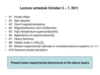
Lecture schedule October 3 – 7, 2011 Present basic experimental phenomena of the above topics Present basic experimental phenomena of the above topics #1 Kondo effect #2 Spin glasses #3 Giant magnetoresistance #4 Magnetoelectrics and multiferroics #5 High temperature superconductivity #6 Applications of superconductivity #7 Heavy fermions #8 Hidden order in URu2Si2 #9 Modern experimental methods in correlated electron systems #10 Quantum phase transitions
# 10 Quantum Phase Transitions:Theoretical driven 1975 … Experimentally first found 1994 … : T = 0 phase transition tuned by pressure, doping or magnetic field [Also quantum well structures] e.g.,3D AF e.g., FL e.g.,2D Heisenberg AF r is the tuning parameter: P, x; H
Critical exponents – thermal (TC) where t = (T – TC)/TC and quantum phase (all at T = 0) 2nd order phase transitions QPT: Δ ~ J|r –rc|zν,ξ-1 ~ Λ|r – rc|ν, Δ ~ξ-z,ћω >> kBT, T = 0 and r & rc finite
Parameters of QPT describing T = 0K singularity, yet they strongly influence the experimental behavior at T > 0 Δ is spectral density fluctuation scale at T = 0 for , e.g., energy of lowest excitation above the ground state or energy gap or qualitative change in nature of frequency spectrum. Δ 0 as r rc. J is microscopic coupling energy. z and ν are the critical exponents. is the diverging characteristic length scale. Λis an inverse length scale or momentum. ω is frequency at which the long-distance degrees of freedomfluctuate. For a purely classical description ħωtyp << kBT with classical critical exponents. Usually interplay of classical (thermal) fluctuations and quantum fluctuations driven by Heisenberg uncertainty principle.
Beyond the T = O phase transition: How about the dynamics at T > 0? eq is thermal equilibration time, i.e., when local thermal equilibrium is established. Two regimes: If Δ> kBT, long equilibration times: τeq>> ħ/kBT classical dynamics If Δ < kBT, short equilibration times: τeq ~ ħ/kBT quantum critical Note dashed crossover lines
Crossover lines, divergences and imaginary time: Some unique properties of QPT
Hypothesis: Black hole in space – time is the quantum critical matter (droplet) at the QCP (T = 0). Material event horizon – separates the electrons into their spin and charge constituents through two new horizons.
Subtle ways of non-temperature tuning QCP: (i) Level crossings/ repulsions and (ii) layer spacing variation in 2D quantum wells Excited state becomes ground state: continuously or gapping: light or frequency tuning. Non-analyticity at gC. Usually 1st order phase transition –.…..NOT OF INTEREST HERE…… Varying green layer thickness changes ferri- magnetic coupling (a) to quantum paramagnet (dimers) with S =1 triplet excitations.
Experimental examples of tuning of QCP: LiHoF4 Ising ferromagnet in transverse magnetic field (H) H┴ induces quantum tunneling between the two states: all ↑↑↑↑ or all ↓↓↓↓. Strong tunneling of transverse spin fluctuations destroys long-range ferromagnetic order at QCP. Note for dilute/disordered case of Li(Y1-xHox )F4 can create a putative quantum spin glass. Bitko et al. PRL(1996)
Solution of quantum Ising model in transverse field where Jg = µH and J exchange coupling: F (here) or AF nonmagnetic ferromagnetic Somewhere (at gC) between these two states there is non-analyticity, i.e., QPT/QCP
Some experimental systems showing QCP at T = 0K with magnetic field, pressue or doping (x) tuning • CoNb2O6 -- quantum Isingin H with short range Heisenberg exchange, not long-range magnetic dipoles of LiHoF4. • TiCuCl3 -- Heisenberg dimers (single valence bond) due to crystal structure, under pressure forms an ordered Neél anitferromagnet via a QPT. • CeCu6-xAux -- heavy fermion antiferromagnet tuned into QPT via pressure, magnetic field and Aux- doping. • YbRh2Si2 -- 70 mK antiferromagnetic to Fermi liquid with tiny fields. Sr3Ru2O7 and URu2Si2 “novel phases”, field-induced, masking QCP. Non-tuned QCP at ambients “serendipity” CeNi2Ge2 YbAlB???. Let’s look in more detail at the first (1994)one CeCu6-xAux.
Ce Cu6-xAux experiments: Low-T specific heat tuned with x(i) x=0, C/T const. Fermi liquid (ii) x=0.05;0.1 logT NFL behavior and (iii) x= 0.15,0.2;0.3 onset of maxima AF order At x = 0.1 as T0 QCP von Löhneysen et al. PRL(1994)
Susceptibility (M/H) vs T at x=0.1 in 0.1T(NFL -> QCP): χ =χo( 1 – a√T ) and in 3T(normal FL): χ = const. Field restores HFL behavior. Pressure also. (1 - a√T) von Löheneysen et al.PRL(1994)
Resistivity vs T field at x=0.1 in 0-field: ρ = ρo+ bT {NFL} but infields: ρ =ρo+ AT2 {FL}. Field restores HFL behavior. von Löhneysen et al. PRL(1994)
T – x phase diagram for CeCu6-xAux in zero field and at ambient pressure. Green arrow is QCP at x=0.1 Pressure and magnetic field
Pressure dependence of C/T as fct.(x,P) where P is the hydrostatic pressure. Note how AFM 0.2 and 0.3 are shifted with P to NFL behavior and 0.1 at 6kbar is HFLiq.
Two “famous” scenarios for QCP (here at x=0.1)(b)local moments are quenched at a finite TK AFM via SDW (c)local moments exist, only vanish at QCP Kondo breakdown Which materials obey scenario (b) or (c)?? W is magnetic coupling between conduction electrons and f-electrons, TN=0 at Wc :QCP
Weak vs strong coupling models for QPT with NFL.Top] From FL to magnetic instability (SDW)Bot] Local magnetic moments (AFM) to Kondo lattice
Many disordered materials-NFL, yet unknown effects of disorder
So what is all this non-Fermi liquid (NFL) behavior? See Steward, RMP (2001 and 2004)
Hertz-PRB(1976), Millis-PRB(1993); Moriya-BOOK(1985) theory of QPT for itinerant fermions. Order parameter(OP) theory from microscopic model for interacting electrons. S is effective action for a field tuned QCP with vector field OP -1 (propagator)and b2i (coefficients) are diagramatically calculated. After intergrating out the the fermion quasiparticles: where |ω|/kz-2 is the damping term of the OP fluct. of el/hole paires at the FS and d = 2 or 3 dims., and z the dynamical critical exponent. Use renormalization-group techniques to study QPT in 2 or 2 dims. for Q vectors that do not span FS. Results depend critically on d and z Predictions of theories for measureable NFL quantities -over-
Predictions of different SF theories: FM & AFM in d & z(a) Millis/Hertz [TN/C Néel/Curie & TI/II crossover T’s](b) Moriya et al.(c) Lonzarich {All NFL behaviors]
Millis/Hertz theory-based T – r (tuning) phase diagram I) Disordered quantum regime-HFLiq., II) perturbed classical regime, III) quantum critical-NFL, and V) magnetically ordered Néel/Curie [SDW] phase transitions. Dashed lines are crossovers.
Summary: Quantum Phase Transitions Apologies being too brief and superficial The end of Lectures
EXP LiHoF4 xxx