Download

1 / 50
510 likes | 809 Views
C H A P T E R 4. Individual and Market Demand. CHAPTER OUTLINE. 4.1 Individual Demand 4.2 Income and Substitution Effects 4.3 Market Demand 4.4 Consumer Surplus 4.5 Network Externalities 4.6 Empirical Estimation of Demand Appendix : Demand Theory—A Mathematical Treatment.

E N D
C H A P T E R 4 Individual and Market Demand CHAPTER OUTLINE 4.1Individual Demand 4.2 Income and Substitution Effects 4.3Market Demand 4.4Consumer Surplus 4.5Network Externalities 4.6Empirical Estimation of Demand Appendix: Demand Theory—A Mathematical Treatment Prepared by: Fernando Quijano, Illustrator
Our analysis of demand proceeds in six steps: • We begin by deriving the demand curve for an individual consumer. • With this foundation, we will examine the effect of a price change in more detail. • Next, we will see how individual demand curves can be aggregated todetermine the market demand curve. • We will go on to show how market demand curves can be used to measurethe benefits that people receive when they consume products, above and beyond the expenditures they make. • We then describe the effects of network externalities—i.e., what happenswhen a person’s demand for a good also depends on the demands of otherpeople. 6. Finally, we will briefly describe some of the methods that economists use to obtain empirical information about demand.
Individual Demand Price Changes 4.1 FIGURE 4.1 EFFECT OF PRICE CHANGES A reduction in the price of food, with income and the price of clothing fixed, causes the consumer to choose a different market basket. In panel (a), the baskets that maximize utility for various prices of food (point A, $2; B, $1; D, $0.50) trace out the price-consumption curve. Part (b) gives the demand curve, which relates the price of food to the quantity demanded. (Points E, G, and H correspond to points A, B, and D, respectively).
The Individual Demand Curve ●price-consumption curve Curve tracing the utility-maximizing combinations of two goods as the price of one changes. ●individual demand curve Curve relating the quantity of a good that a single consumer will buy to its price. The individual demand curve has two important properties: 1. The level of utility that can be attained changes as we move along the curve. 2.At every point on the demand curve, the consumer is maximizing utility by satisfying the condition that the marginal rate of substitution (MRS) of food for clothing equals the ratio of the prices of food and clothing. Income Changes ●income-consumption curve Curve tracing the utility-maximizing combinations of two goods as a consumer’s income changes.
FIGURE 4.2 EFFECT OF INCOME CHANGES An increase in income, with the prices of all goods fixed, causes consumers to alter their choice of market baskets. In part (a), the baskets that maximize consumer satisfaction for various incomes (point A, $10; B, $20; D, $30) trace out the income-consumption curve. The shift to the right of the demand curve in response to the increases in income is shown in part (b). (Points E, G, and H correspond to points A, B, and D, respectively.)
Normal versus Inferior Goods FIGURE 4.3 AN INFERIOR GOOD An increase in a person’s income can lead to less consumption of one of the two goods being purchased. Here, hamburger, though a normal good between A and B, becomes an inferior good when the income-consumption curve bends backward between B and C.
Engel Curves ●Engel curve Curve relating the quantity of a good consumed to income. FIGURE 4.4 ENGLE CURVES Engel curves relate the quantity of a good consumed to income. In (a), food is a normal good and the Engel curve is upward sloping. In (b), however, hamburger is a normal good for income less than $20 per month and an inferior good for income greater than $20 per month.
EXAMPLE 4.1 CONSUMER EXPENDITURES IN THE UNITED STATES We can derive Engel curves for groups of consumers. This information is particularly useful if we want to see how consumer spending varies among different income groups.
EXAMPLE 4.1 CONSUMER EXPENDITURES IN THE UNITED STATES FIGURE 4.5 ENGEL CURVES FOR U.S. CONSUMERS Average per-household expenditures on rented dwellings, health care, and entertainment are plotted as functions of annual income. Health care and entertainment are normal goods, as expenditures increase with income. Rental housing, however, is an inferior good for incomes above $30,000.
Substitutes and Complements Two goods are substitutes if an increase in the price of one leads to an increase in the quantity demanded of the other. Two goods are complements if an increase in the price of one good leads to a decrease in the quantity demanded of the other. Two goods are independent if a change in the price of one good has no effect on the quantity demanded of the other. The fact that goods can be complements or substitutes suggests that when studying the effects of price changes in one market, it may be important to look at the consequences in related markets.
4.2 Income and Substitution Effects A fall in the price of a good has two effects: • Consumers will tend to buy more of the good that has become cheaper and less of those goods that are now relatively more expensive. This response to a change in the relative prices of goodsis called the substitution effect. • Because one of the goods is now cheaper, consumers enjoy anincrease in real purchasing power. The change in demand resultingfrom this change in real purchasing power is called the income effect.
substitution effect Change in consumption of a good associated with a change in its price, with the level of utility held constant. Substitution Effect Income Effect • income effect Change in consumption of a good resulting from an increase in purchasing power, with relative prices held constant. In Figure 4.6, the total effect of a change in price is given theoretically by the sum of the substitution effect and the income effect: Total Effect (F1F2) = Substitution Effect (F1E) + Income Effect (EF2)
FIGURE 4.6 INCOME AND SUBSTITUTION EFFECTS: NORMAL GOOD A decrease in the price of food has both an income effect and a substitution effect. The consumer is initially at A, on budget line RS. When the price of food falls, consumption increases by F1F2 as the consumer moves to B. The substitution effect F1E (associated with a move from A to D) changes the relative prices of food and clothing but keeps real income (satisfaction) constant. The income effect EF2 (associated with a move from D to B) keeps relative prices constant but increases purchasing power. Food is a normal good because the income effect EF2 is positive.
FIGURE 4.7 INCOME AND SUBSTITUTION EFFECTS: INFERIOR GOOD The consumer is initially at A on budget line RS. With a decrease in the price of food, the consumer moves to B. The resulting change in food purchased can be broken down into a substitution effect, F1E (associated with a move from A to D), and an income effect, EF2 (associated with a move from D to B). In this case, food is an inferior good because the income effect is negative. However, because the substitution effect exceeds the income effect, the decrease in the price of food leads to an increase in the quantity of food demanded.
A Special Case: The Giffen Good • Giffen good Good whose demand curve slopes upward becausethe (negative) income effect is larger than the substitution effect. FIGURE 4.8 UPWARD-SLOPING DEMAND CURVE: THE GIFFEN GOOD When food is an inferior good, and when the income effect is large enough to dominate the substitution effect, the demand curve will be upward-sloping. The consumer is initially at point A, but, after the price of food falls, moves to B and consumes less food. Because the income effect F2F1 is larger than the substitution effect EF2, the decrease in the price of food leads to a lower quantity of food demanded.
EXAMPLE 4.2 THE EFFECTS OF A GASOLINE TAX FIGURE 4.9 EFFECT OF A GASOLINE TAX WITH A RE BATE A gasoline tax is imposed when the consumer is initially buying 1200 gallons of gasoline at point C. After the tax takes effect, the budget line shifts from AB to AD and the consumer maximizes his preferences by choosing E, with a gasoline consumption of 900 gallons. However, when the proceeds of the tax are rebated to the consumer, his consumption increases somewhat, to 913.5 gallons at H. Despite the rebate program, the consumer’s gasoline consumption has fallen, as has his level of satisfaction.
Market Demand 4.3 ●market demand curve Curve relating the quantity of a goodthat all consumers in a market will buy to its price. From Individual to Market Demand
FIGURE 4.10 SUMMING TO OBTAIN A MARKET DEMAND CURVE The market demand curve is obtained by summing our three consumers’ demand curves DA, DB, and DC. At each price, the quantity of coffee demanded by the market is the sum of the quantities demanded by each consumer. At a price of $4, for example, the quantity demanded by the market (11 units) is the sum of the quantity demanded by A (no units), B (4 units), and C (7 units).
Two points should be noted: • The market demand curve will shift to the right as more consumers enterthe market. • Factors that influence the demands of many consumers will also affect market demand. The aggregation of individual demands into market becomes important in practice when market demands are built up from the demands of different demographic groups or from consumers located in different areas.
Elasticity of Demand Denoting the quantity of a good by Q and its price by P, the price elasticity of demand is (4.1) INELASTIC DEMAND When demand is inelastic, the quantity demanded is relatively unresponsive to changes in price. As a result, total expenditure on the product increases when the price increases. ELASTIC DEMAND When demand is elastic, total expenditure on the product decreases as the price goes up.
ISOELASTIC DEMAND • isoelastic demand curve Demand curve with a constant price elasticity. FIGURE 4.11 UNIT-ELASTIC DEMAND CURVE When the price elasticity of demand is −1.0 at every price, the total expenditure is constant along the demand curve D.
Speculative Demand ●speculative demand Demand driven not by the direct benefits one obtains from owning or consuming a good but instead by an expectation that the price of the good will increase.
EXAMPLE 4.3 THE AGGREGATE DEMAND FOR WHEAT Domestic demand for wheat is given by the equation QDD = 1430 − 55P where QDD is the number of bushels (in millions) demanded domestically, and P is the price in dollars per bushel. Export demand is given by QDE = 1470 − 70P where QDE is the number of bushels (in millions) demanded from abroad. To obtain the world demand for wheat, we set the left side of each demand equation equal to the quantity of wheat. We then add the right side of the equations, obtaining QDD + QDE = (1430 − 55P) + (1470 − 70P) = 2900 − 125P
EXAMPLE 4.3 THE AGGREGATE DEMAND FOR WHEAT FIGURE 4.12 THE AGGREGATE DEMAND FOR WHEAT The total world demand for wheat is the horizontal sum of the domestic demand AB and the export demand CD. Even though each individual demand curve is linear, the market demand curve is kinked, reflecting the fact that there is no export demand when the price of wheat is greater than about $21 per bushel.
EXAMPLE 4.4 THE DEMAND FOR HOUSING There are significant differences in price and income elasticities of housing demand among subgroups of the population. In recent years, the demand for housing has been partly driven by speculative demand. Speculative demand is driven not by the direct benefits one obtains from owning a home but instead by an expectation that the price will increase.
EXAMPLE 4.5 THE LONG-RUN DEMAND FOR GASOLINE Would higher gasoline prices reduce gasoline consumption? Figure 4.13 provides a clear answer: Most definitely. FIGURE 4.13 GASOLINE PRICES AND PER CAPITA CONSUMPTION IN 10 COUNTRIES The graph plots per capita consumption of gasoline versus the price per gallon (converted to U.S. dollars) for 10 countries over the period 2008 to 2010. Each circle represents the population of the corresponding country.
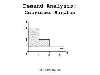
Consumer Surplus 4.4 ●consumer surplusDifference between what a consumer is willing to pay for a good and the amount actually paid. Consumer Surplus and Demand FIGURE 4.14 CONSUMER SURPLUS Consumer surplus is the total benefit from the consumption of a product, less the total cost of purchasing it. Here, the consumer surplus associated with six concert tickets (purchased at $14 per ticket) is given by the yellow-shaded area: $6 + $5 + $4 + $3 + $2 + $1 = $21
FIGURE 4.15 CONSUMER SURPLUS GENERALIZED For the market as a whole, consumer surplus is measured by the area under the demand curve and above the line representing the purchase price of the good. Here, the consumer surplus is given by the yellow-shaded triangle and is equal to 1/2 ($20 − $14) 6500 = $19,500. APPLYING CONSUMER SURPLUS Consumer surplus has important applications in economics. When added over many individuals, it measures the aggregate benefit that consumers obtain from buying goods in a market. When we combine consumer surplus with the aggregate profits that producers obtain, we can evaluate both the costs and benefits not only of alternative market structures, but of public policies that alter the behavior of consumers and firms in those markets.
EXAMPLE 4.6 THE VALUE OF CLEAN AIR Although there is no actual market for clean air, people do pay more for houses where the air is clean than for comparable houses in areas with dirtier air. FIGURE 4.16 VALUING CLEANER AIR The yellow-shaded triangle gives the consumer surplus generated when air pollution is reduced by 5 parts per 100 million of nitrogen oxide at a cost of $1000 per part reduced. The surplus is created because most consumers are willing to pay more than $1000 for each unit reduction of nitrogen oxide.
Network Externalities 4.5 ●network externality When each individual’s demand depends on the purchases of other individuals. A positive network externality exists if the quantity of a good demanded by a typical consumer increases in response to the growth in purchases of other consumers. If the quantity demanded decreases, there is a negative network externality. Positive Network Externalities ●bandwagon effect Positive network externality in which a consumer wishes to possess a good in part because others do.
FIGURE 4.17 POSITIVE NETWORK EXTERNALITY With a positive network externality, the quantity of a good that an individual demands grows in response to the growth of purchases by other individuals. Here, as the price of the product falls from $30 to $20, the bandwagon effect causes the demand for the good to shift to the right, from D40 to D80.
Negative Network Externalities ●snob effect Negative network externality in which a consumer wishes to own an exclusive or unique good. FIGURE 4.18 NEGATIVE NETWORK EXTERNALITY: SNOB EFFECT The snob effect is a negative network externality in which the quantity of a good that an individual demands falls in response to the growth of purchases by other individuals. Here, as the price falls from $30,000 to $15,000 and more people buy the good, the snob effect causes the demand for the good to shift to the left, from D2 to D6.
EXAMPLE 4.7 FACEBOOK By early 2011, with over 600 million users, Facebook became the world’s second most visited website (after Google). A strong positive network externality was central to Facebook’s success. Network externalities have been crucial drivers for many modern technologies over many years.
Empirical Estimation of Demand 4.6 The Statistical Approach to Demand Estimation (4.2) Using the data in the table and the least squares method, the demand relationship is:
FIGURE 4.19 ESTIMATING DEMAND Price and quantity data can be used to determine the form of a demand relationship. But the same data could describe a single demand curve D or three demand curves d1, d2, and d3 that shift over time.
The Form of the Demand Relationship The price elasticity for equals: (4.3) We often find it useful to work with the isoelastic demand curve, in which the price elasticity and the income elasticity are constant. When written in its log-linear form, an isoelastic demand curve appears as follows: (4.4) Suppose that P2 represents the price of a second good—one which is believed to be related to the product we are studying. We can then write the demand function in the following form: When b2, the cross-price elasticity, is positive, the two goods are substitutes; when b2 is negative, the two goods are complements.
EXAMPLE 4.8 THE DEMAND FOR READY-TO-EAT CEREAL The acquisition of Shredded Wheat cereals of Nabiscoby Post Cereals raised the question of whether Postwould raise the price of Grape Nuts, or the price ofNabisco’s Shredded Wheat Spoon Size. One important issue was whether the two brands wereclose substitutes for one another. If so, it would be moreprofitable for Post to increase the price of Grape Nuts after rather than before the acquisition because the lostsales from consumers who switched away from Grape Nuts would be recovered to the extent that they switched to the substitute product. The substitutability of Grape Nuts and Shredded Wheat can be measured by the cross-price elasticity of demand for Grape Nuts with respect to the price of Shredded Wheat. One isoelastic demand equation appeared in the following log-linear form: The demand for Grape Nuts is elastic, with a price elasticity of about −2. Income elasticity is 0.62. the cross-price elasticity is 0.14. The two cereals are not very close substitutes.
Interview and Experimental Approaches toDemand Determination Another way to obtain information about demand is through interviews.This approach, however, may not succeed when people lack information or interest or even want to mislead the interviewer. In direct marketing experiments, actual sales offers are posed to potential customers. An airline, for example, might offer a reduced price on certain flights for six months, partly to learn how the price change affects demand for flights and partly to learn how competitors will respond. Alternatively, a cereal company might test market a new brand, with some potential customers being given coupons ranging in value from 25 cents to $1 per box. The response to the coupon offer tells the company the shape of the underlying demand curve. Direct experiments are real, not hypothetical, but even so, problems remain. The wrong experiment can be costly, and the firm cannot be entirely sure that these increases resulted from the experimental change; other factors probably changed at the same time. Moreover, the response to experiments—which consumers often recognize as short-lived—may differ from the response to permanent changes. Finally, a firm can afford to try only a limited number of experiments.
Appendix to Chapter 4 Demand Theory—A Mathematical Treatment Utility Maximization Suppose, for example, that Bob’s utility function is given by U(X, Y) = log X + log Y, where X is used to represent food and Y represents clothing. In that case, the marginal utility associated with the additional consumption of X is given by the partial derivative of the utility function with respect to good X. Here, MUX, representing the marginal utility of good X, is given by The consumer’s optimization problem may be written as (A4.1) subject to the constraint that all income is spent on the two goods: (A4.2)
The Method of Lagrange Multipliers ●method of Lagrange multipliersTechnique to maximize or minimize a function subject to one or more constraints. ●LagrangianFunction to be maximized or minimized, plus a variable (the Lagrange multiplier) multiplied by the constraint. Stating the Problem First, we write the Lagrangian for the problem. (A4.3) Note that we have written the budget constraint as
Differentiating the Lagrangian We choose values of X and Y that satisfy the budget constraint, then the second term in equation (A4.3) will be zero. By differentiating with respect to X, Y, and l and then equating the derivatives to zero, we can obtain the necessary conditions for a maximum. (A4.4) Solving the Resulting Equations The three equations in (A4.4) can be rewritten as
The Equal Marginal Principle We combine the first two conditions above to obtain the equal marginal principle: (A4.5) To optimize, the consumer must get the same utility from the last dollar spent by consuming either X or Y. To characterize the individual’s optimum in more detail, we can rewrite the information in (A4.5) to obtain (A4.6) Marginal Rate of Substitution If U* is a fixed utility level, the indifference curve that corresponds to that utility level is given by (A4.7) Rearranging, (A4.8)
Marginal Utility of Income The Lagrange multiplier l represents the extra utility generated whenthe budget constraint is relaxed. To show how the principle works, we differentiate the utility function U(X, Y) totally with respect to I: (A4.9) Because any increment in income must be divided between the two goods, it follows that (A4.10) Substituting from (A4.5) into (A4.9), we get (A4.11) Substituting from (A4.10) into (A4.11), we get (A4.12) Thus the Lagrange multiplier is the extra utility that results from an extra dollar of income.
An Example ●Cobb-Douglas utility function Utility function U(X,Y) = XaY1−a,where X and Y are two goods and a is a constant. The Cobb-Douglas utility function can be represented in two forms: and To find the demand functions for X and Y, given the usual budget constraint, we first write the Lagrangian: Now differentiating with respect to X, Y, and l and setting the derivatives equal to zero, we obtain
The first two conditions imply that (A4.13) (A4.14) Combining these expressions with the last condition (the budget constraint) gives us or Now we can substitute this expression for λ back into (A4.13) and (A4.14) to obtain the demand functions:
Duality in Consumer Theory ●duality Alternative way of looking at the consumer’s utilitymaximization decision: Rather than choosing the highest indifference curve, given a budget constraint, the consumer chooses the lowest budget line that touches a given indifference curve. Minimizing the cost of achieving a particular level of utility: Minimize subject to the constraint that The corresponding Lagrangian is given by (A4.15) Differentiating with respect to X, Y, and μ and setting the derivatives equal to zero, we find the following necessary conditions for expenditure minimization: and
By solving the first two equations, and recalling (A4.5), we see that Because it is also true that Here we use the exponential form of the Cobb-Douglas utility function, In this case, the Lagrangian is given by (A4.16) Differentiating with respect to X, Y, and μ and setting the derivatives equal to zero, we find the following necessary conditions for expenditure minimization: Multiplying the first equation by X and the second by Y and adding, we get First, we let I be the cost-minimizing expenditure. Then it follows that μ = I/U*. Substituting in the equations above, we obtain the same demand equations as before:
Income and Substitution Effects It is important to distinguish that portion of any price change thatinvolves movement along an indifference curve from that portion which involves movement to a different indifference curve (and therefore a change in purchasing power). We denote the change in X that results from a unit change in the price of X, holding utility constant, by The total change in the quantity demanded of X resulting from a unit change in PX is (A4.17) The first term on the right side of equation (A4.17) is the substitution effect (because utility is fixed); the second term is the income effect (because income increases). From the consumer’s budget constraint, , we know by differentiation that (A4.18)
It is customary to write the income effect as negative (reflecting a loss of purchasing power) rather than as a positive. Equation (A4.17) then appears as follows: (A4.19) In this new form, called the Slutsky equation, the first term represents the substitution effect: the change in demand for good X obtained by keeping utility fixed. The second term is the income effect: the change in purchasing power resulting from the price change times the change in demand resulting from a change in purchasing power. ●Slutsky equation Formula for decomposing the effects of a price change into substitution and income effects.
●Hicksian substitution effect Alternative to the Slutsky equation for decomposing price changes without recourse to indifference curves. FIGURE A4.1 HICKSIAN SUBSTITUTION EFFECT The individual initially consumes market basket A. A decrease in the price of food shifts the budget line from RS to RT. If a sufficient amount of income is taken away to make the individual no better off than he or she was at A, two conditions must be met: The new market basket chosen must lie on line segment B′T' of budget line R′T'(which intersects RS to the right of A), and the quantity of food consumed must be greater than at A.