Download
1 / 42
420 likes | 504 Views
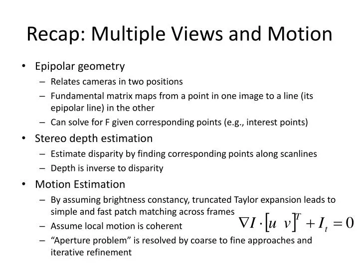
Recap: Multiple Views and Motion. Epipolar geometry Relates cameras in two positions Fundamental matrix maps from a point in one image to a line (its epipolar line) in the other Can solve for F given corresponding points (e.g., interest points) Stereo depth estimation

E N D
Recap: Multiple Views and Motion • Epipolar geometry • Relates cameras in two positions • Fundamental matrix maps from a point in one image to a line (its epipolar line) in the other • Can solve for F given corresponding points (e.g., interest points) • Stereo depth estimation • Estimate disparity by finding corresponding points along scanlines • Depth is inverse to disparity • Motion Estimation • By assuming brightness constancy, truncated Taylor expansion leads to simple and fast patch matching across frames • Assume local motion is coherent • “Aperture problem” is resolved by coarse to fine approaches and iterative refinement
Machine Learning Computer Vision James Hays, Brown Slides: Isabelle Guyon, Erik Sudderth, Mark Johnson,Derek Hoiem Photo: CMU Machine Learning Department protests G20
It is a rare criticism of elite American university students that they do not think big enough. But that is exactly the complaint from some of the largest technology companies and the federal government. At the heart of this criticism is data. Researchers and workers in fields as diverse as bio-technology, astronomy and computer science will soon find themselves overwhelmed with information. The next generation of computer scientists has to think in terms of what could be described as Internet scale. New York Times Training to Climb an Everest of Digital Data. By Ashlee Vance. Published: October 11, 2009
Machine learning: Overview • Core of ML: Making predictions or decisions from Data. • This overview will not go in to depth about the statistical underpinnings of learning methods. We’re looking at ML as a tool. Take CS 142: Introduction to Machine Learning to learn more.
Impact of Machine Learning • Machine Learning is arguably the greatest export from computing to other scientific fields.
Machine Learning Applications Slide: Isabelle Guyon
Image Categorization Training Training Labels Training Images Image Features Classifier Training Trained Classifier
Image Categorization Training Training Labels Training Images Image Features Classifier Training Trained Classifier Testing Prediction Image Features Trained Classifier Outdoor Test Image
Example: Scene Categorization • Is this a kitchen?
Image features Training Training Labels Training Images Image Features Classifier Training Trained Classifier
General Principles of Representation • Coverage • Ensure that all relevant info is captured • Concision • Minimize number of features without sacrificing coverage • Directness • Ideal features are independently useful for prediction
Image representations • Templates • Intensity, gradients, etc. • Histograms • Color, texture, SIFT descriptors, etc.
Classifiers Training Training Labels Training Images Image Features Classifier Training Trained Classifier
Learning a classifier Given some set of features with corresponding labels, learn a function to predict the labels from the features x x x x x x x o x o o o o x2 x1
Many classifiers to choose from • SVM • Neural networks • Naïve Bayes • Bayesian network • Logistic regression • Randomized Forests • Boosted Decision Trees • K-nearest neighbor • RBMs • Etc. Which is the best one?
One way to think about it… • Training labels dictate that two examples are the same or different, in some sense • Features and distance measures define visual similarity • Classifiers try to learn weights or parameters for features and distance measures so that visual similarity predicts label similarity
Claim: The decision to use machine learning is more important than the choice of a particular learning method. If you hear somebody talking of a specific learning mechanism, be wary (e.g. YouTube comment "Oooh, we could plug this in to a Neural networkand blah blahblah“)
Dimensionality Reduction • PCA, ICA, LLE, Isomap • PCA is the most important technique to know. It takes advantage of correlations in data dimensions to produce the best possible lower dimensional representation, according to reconstruction error. • PCA should be used for dimensionality reduction, not for discovering patterns or making predictions. Don't try to assign semantic meaning to the bases.
Clustering example: image segmentation Goal: Break up the image into meaningful or perceptually similar regions
Segmentation for feature support 50x50 Patch 50x50 Patch Slide: Derek Hoiem
Segmentation for efficiency [Felzenszwalb and Huttenlocher 2004] [Shi and Malik 2001] Slide: Derek Hoiem [Hoiem et al. 2005, Mori 2005]
Segmentation as a result Rother et al. 2004
Types of segmentations Oversegmentation Undersegmentation Multiple Segmentations
Clustering: group together similar points and represent them with a single token Key Challenges: 1) What makes two points/images/patches similar? 2) How do we compute an overall grouping from pairwise similarities? Slide: Derek Hoiem
Why do we cluster? • Summarizing data • Look at large amounts of data • Patch-based compression or denoising • Represent a large continuous vector with the cluster number • Counting • Histograms of texture, color, SIFT vectors • Segmentation • Separate the image into different regions • Prediction • Images in the same cluster may have the same labels Slide: Derek Hoiem
How do we cluster? • K-means • Iteratively re-assign points to the nearest cluster center • Agglomerative clustering • Start with each point as its own cluster and iteratively merge the closest clusters • Mean-shift clustering • Estimate modes of pdf • Spectral clustering • Split the nodes in a graph based on assigned links with similarity weights
Clustering for Summarization Goal: cluster to minimize variance in data given clusters • Preserve information Cluster center Data Whether xj is assigned to ci Slide: Derek Hoiem
K-means algorithm 1. Randomly select K centers 2. Assign each point to nearest center 3. Compute new center (mean) for each cluster Illustration: http://en.wikipedia.org/wiki/K-means_clustering
K-means algorithm 1. Randomly select K centers 2. Assign each point to nearest center Back to 2 3. Compute new center (mean) for each cluster Illustration: http://en.wikipedia.org/wiki/K-means_clustering
K-means • Initialize cluster centers: c0 ; t=0 • Assign each point to the closest center • Update cluster centers as the mean of the points • Repeat 2-3 until no points are re-assigned (t=t+1) Slide: Derek Hoiem
K-means: design choices • Initialization • Randomly select K points as initial cluster center • Or greedily choose K points to minimize residual • Distance measures • Traditionally Euclidean, could be others • Optimization • Will converge to a local minimum • May want to perform multiple restarts
How to evaluate clusters? • Generative • How well are points reconstructed from the clusters? • Discriminative • How well do the clusters correspond to labels? • Purity • Note: unsupervised clustering does not aim to be discriminative Slide: Derek Hoiem
How to choose the number of clusters? • Validation set • Try different numbers of clusters and look at performance • When building dictionaries (discussed later), more clusters typically work better Slide: Derek Hoiem
K-Means pros and cons • Pros • Finds cluster centers that minimize conditional variance (good representation of data) • Simple and fast* • Easy to implement • Cons • Need to choose K • Sensitive to outliers • Prone to local minima • All clusters have the same parameters (e.g., distance measure is non-adaptive) • *Can be slow: each iteration is O(KNd) for N d-dimensional points • Usage • Rarely used for pixel segmentation
Building Visual Dictionaries • Sample patches from a database • E.g., 128 dimensional SIFT vectors • Cluster the patches • Cluster centers are the dictionary • Assign a codeword (number) to each new patch, according to the nearest cluster
Examples of learned codewords Most likely codewords for 4 learned “topics” EM with multinomial (problem 3) to get topics http://www.robots.ox.ac.uk/~vgg/publications/papers/sivic05b.pdf Sivic et al. ICCV 2005