Mesoscale Atmospheric Predictability

1. Mesoscale Atmospheric Predictability Martin Ehrendorfer Institut für Meteorologie und Geophysik Universität Innsbruck Presentation at 14th ALADIN Workshop 1-4 June 2004 Innsbruck, Austria 3 June 2004 http://www2.uibk.ac.at/meteo http://www.zamg.ac.at/workshop2004/

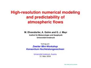
2. Mesoscale Atmospheric Predictability Outline 1 Predictability: error growth 2 Global Models: doubling times 3 Singular Vectors: assessing growth 4 Mesoscale Studies: moist physics 5 Ensemble Prediction: sampling 6 Conclusions

3. 1 T+36; 02/06/2004/00

4. T+12 – T+24 T+36 – T+48 02/06/2004/12 01/06/2004/12 T+24 – T+36 T+48 – T+60 02/06/2004/00 03/06/2004/00

5. - intrinsic error growth - chaotic: to extent to which model and atmosphere correspond

8. reduced D+1 error better consistency reduced gap between error and difference amplification of 1-day forecast error, 1.5 days A. Simmons, ECMWF

9. nonlinearity of dynamics and instability with respect to small perturbations  sensitive dependence on present condition chaos irregularity and nonperiodicity unpredictability and error growth

10. 2 Tribbia/Baumhefner 2004 all scales DAY 0 55 m 25m large scales small scales 10 m 45m 10m 15m 10m

11. Tribbia/Baumhefner 2004 all scales DAY 1 85m large scales 85m small scales 10 m 10m 75m 10m 75m

12. all scales Tribbia/Baumhefner 2004 DAY 3 small scales large scales 20 m

13. similarity of spectra at day 3  spectrally local error reduction will not help only small- scale error

14. error growth to due resolution differences (against T170): D+1 error T42 = 10 x D+1 error T63 = 10 x D+1 error T106

15. even at T42 the D+1 truncation error growth has not exceeded D+1 IC T106 growth T106 truncation error growth is one order of magnitude smaller than D+1 T106 IC error growth need IC/10 before going beyond T106 [ IC analysis error growth exponential ] T106 Tribbia Baumhefner 2004

16. - sensitive dependence on i.c. - preferred directions of growth Lorenz 1984 model Ehrendorfer 1997

17. 3 R.M. Errico SVs / HSVs -> fastest growing directions: account for in initial condition stability of the flow

18. psi´ at 500 hPa Optimized TL error growth data assimilation, stability, error dynamics French storm tau_d = 4.9 h

19. lambda = 56.6 tau_d =4.1 h Ehrendorfer/Errico 1995 MAMS - DRY TE-Norm

20. Mesoscale Adjoint Modeling SystemMAMS2 PE with water vapor (B grid) Bulk PBL (Deardorff) Stability-dependent vertical diffusion (CCM3) RAS scheme (Moorthi and Suarez) Stable-layer precipitation Dx=80 km 20-level configuration (d sigma=0.05) Relaxation to lateral boundary condition 12-hour optimization for SVs 4 synoptic cases moist TLM (Errico and Raeder 1999 QJ)

22. Lorenz 1969 Tribbia/Baumhefner 2004 errors in small scales propagate upscale … in spectral space small-scale errors grow and … contaminate … larger scale

23. grad_x J = M^T grad_y J M R.M. Errico

24. Example Sensitivity Field 36-h sensitivity of surface pressure at P to Z-perturb. 10m at M  1 Pa at P Errico and Vukicevic 1992 MWR Contour interval 0.02 Pa/m M=0.1 Pa/m

25. 4 MOIST PHYSICS initial- and final-time norms E -> E E_m -> E V_d -> E V_d -> P V_m -> E V_m -> P A larger value of E can be produced with an initial constraint V_m=1 compared with V_d=1. (hypothetical norm comparison: “larger E with E_m=1 compared with V_d=1“) Errico et al. 2004 QJ MAMS - MOIST

26. t_d = 2.5 h t_d = 2 h moisture perturbations more effective than dry perturbations to maximize E larger than E_m-> E and V_d->E Doubling time:t_d= OTI * ln 2 / ln l has no vertical scaling

27. r= 0.81 -> E -> P initial time case S2 V_d -> SV2 SV1 v´  r=0.76 q´ V_m -> SV2 SV1  large r: similar structures are optimal for maximizing both E and P highly correlated with T´ of SV2 for V_d -> E

28. Perturbations in Different Fields Can Produce the Same Result 12-hour v TLM forecasts Initial u, v, T, ps Perturbation Initial q Perturbation   Errico et al. QJRMS 2004 H=c_p T + L q condensational heating

29. summarizing comments on moist-norm SV-study: - moisture perturbations alone may achieve larger E than dry perturbations - given same initial constraint, similar structures can be optimal for maximizing E and P in most cases however: structures are different - dry-only and moist-only SVs may lead to nearly identical final-time fields (inferred dependence on H); q converts to T (diabatic heating) through nonconvective precipitation [-nonlinear relevance: TLD vs NLD may match closely (2 g/kg) ] [- sensitivity of non-convective precipitation not universally dominant ]

30. 5 Ensemble Prediction -generate perturbations from (partial) knowledge of analysis error covariance P^a -methodology on the basis of SV -“SV-based sampling technique“

34. QG TE SV spectrum 1642 = 13% lambda_1=33.47 T45/L6 lambda= 0.0212

35. 169 SVs growing out of 4830 (dry balanced norm) i.e. 3.5% of phase space

36. TD and TM curves: 169 (dry) and 175 (wet) growing SVs included for reference (Errico et al. 2001)

37. height correlations 500 hPa derived from ensemble Integrations (D+4) operational EPS (N=25) sampling, N=25, M=50 sampling, N=50, M=100 (Beck 2003)

38. Mesoscale Atmospheric Predictability Summary Intrinsic Error Growth limited predictability (nonlinearity) presence of analysis error Predictability rapid doubling of analysis error account for fastest error growth: SV dynamics importance of lower troposphere insight into growth mechanisms initial moisture perturbations Ensemble Prediction generation of perturbations: sampling SV relation to analysis error: nonmodal IC growth