Download
1 / 37
370 likes | 455 Views
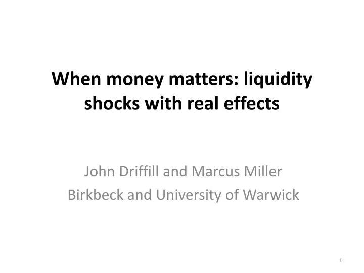
When money matters: liquidity shocks with real effects . John Driffill and Marcus Miller Birkbeck and University of Warwick. Financial boom… ( Note: US GDP is about $14 trillion).

E N D
When money matters: liquidity shocks with real effects John Driffill and Marcus Miller Birkbeck and University of Warwick
Followed by bust: UK recession (dark blue) relative to earlier recessions(dark brown is 1930s; green and yellow follow oil shocks; light brown follows bursting of housing bubble:)
Call for integration of financial factors into real models • In ‘The Great Moderation, the Great Panic and the Great Contraction’ Charlie Bean (2009) calls for further research on financial factors as an urgent priority. • In fact, Kiyotaki and Moore (2008) have developed a ‘workhorse model of money and liquidity’ where liquidity constraints can affect investment and the economy. • With flex-prices and full employment, their focus is on the supply side. • Simulations of such a model by FRBNY- in conjunction with Kiyotaki - in a fix-price environment produce dramatic results for liquidity shocks for aggregate demand.
Background: growth and investment • Before considering how financial factors may affect investment, we look at three real models of capital accumulation • The simplified Solow model of growth • Neoclassical optimising model • Tobin’s q –theory of investment • Reference • Acemoglou, Daron. Introduction to Modern Economic Growth. Princeton Univ Press
Effect of a liquidity shock in US that lasts 10 quarters, Del Negro et al. (2009) – with analytical equivalent from Driffill and Miller (2010) DM
The Simple Solow Growth Model (with Fixed Technology and Exponential Depreciation) y y, output per head Shading shows depreciation c, consumption per head k° = 0 k(o) • k* k, capital per head k k*
Neoclassical growth model:high marginal productivity of capital encourages savings c, consumption per head c° = 0 c y, output per head k° = 0 k(o) • k* k, capital per head • f´(k * )=θ
Dynamics of K and q: phase diagram Asset price stationary q°= 0 Equity Price q K°= 0 U Zero net investment S E S U Capital Stock K K(0) K*
Kiyotaki and Moore (2008): “Liquidity, Business Cycles, and Monetary Policy” • Assets involved: Money and equity • Money is liquid • Equity is not (completely) liquid • only a fraction of holdings can be sold each period • only a fraction of newly produced capital goods can be financed by issuing new equity
Workers – not the focus of attention • Rational and forward-looking, but credit constrained (no borrowing) • Do not have ‘ideas’ for investment • Can hold money and equity if they choose • But choose to spend all they get on consumption and save nothing • So consumption equals wages
Entrepreneurs – play central role, manage production and invest and hold assets • May (prob π) or may not (prob 1-π) have an idea for a profitable investment • Those with no ideas (no investment) • Consume • Save in form of money and equity holdings • Those with an idea (Investors) • Buy new capital goods • Issue equity against them • Use money, other equity holdings, and current income to finance investment
Investment Entrepreneurs can only finance investment using money, selling existing equity claims to others, raising equity on new capital, and spending out of current income
Liquidity constraints on investment • Entrepreneurs can raise equity against up to a fraction θof new investment. • They can sell off a fraction φt of pre-existing equity (theirs and others) nt • Money is perfectly liquid
Entrepreneur’s budget constraint • Budget: • p – price of money; q – equity price • λ – 1-depreciation rate • n equity held by entrepreneur • Objective - max exp U:
Production • CRS / C-D production function, capital and labour • KM: wage clears labour market • DM: fix money wage and price level – entrepreneurs keep the surplus
Investment and Aggregate (Net) Demand Investment demand . Entrepreneurs’ income equals their demand (GM equilibrium)
Basic structure of KM model • 3 equations :Investment Demand, Aggregate Demand (C+I) and Portfolio Balance, between money and shares. • 3 unknowns: price level, Tobin’s q, and K. • Two regimes : • Flex-price: full employment via Pigou effect determines the price level. • Fix-price: agg demand determines employment. • What about K and q?
Stationary conditions for K and q. • The Investment equation and Portfolio Balance determine evolution of K and q. • Stationarity for K is when all capital spending is for Replacement Investment, on upward sloping RI schedule in K,q space. • Stationarity for q, is on downward sloping AM equilibrium schedule where there are no capital gains.
Flex-price comparative statics as in KM (2008): φ increases, liquidity driven expansion,
Fix price comparative statics DM (2010): tightening liquidity shifts RI and AM to left
Dynamics: stock market fall leading to recession – or recovery if shock is to be reversed
Fix price macro • If prices are inflexible downward, there will be no Pigou effect to stabilise aggregate demand in the face of a fall of investment • A fall in demand will contract employment if the real wage is determined by bargaining, as argued for the UK in Layard and Nickell, Alan Manning. • Graphical representation follows of how liquidity contraction can cut income conditional on K and q.
Calibration using FRBNY parameters (qtly) • φ = 0.13 (fraction of existing assets an entrepreneur can sell); • discount factor β = 0.99; • fraction of new capital against which an entrepreneur can raise equity, θ = 0.13; • probability of an entrepreneur having an idea for an investment, π = 0.075; • the quarterly survival rate of the capital stock λ = 0.975 • [ our base case steady state: q = 1.12, r = 0.0374, • Mp/K =0.1171, K = 152.5, y =17.26]
Figure 6. Numerical Results from DM simulation using FRBNY parameters
Table 2. Impact effects of a 20% cut in ϕ for different lengths of time
Figure 9. Bubble collapse preceding liquidity shock: like 1929
Conclusion • Switching from a flex-price to a fix-price framework means that demand failures can emerge after a liquidity shock. • AM and RI offer simple analytical treatment of impact and dynamic effects. • Adding bubble might help explain the origin of the shock- it’s when the bubble bursts • Need to add financial intermediaries to get to the heart of the matter
References • Acemoglou, Daron. Introduction to Modern Economic Growth. Princeton Univ Press • Del Negro, Marco, GautiEggertsson, Andrea Ferrero and NobuhiroKiyotaki (2009). ‘The Great Escape? A Quantitative Evaluation of the Fed's Non-Standard Policies.’ FRBNY working paper. • Dale, Spencer (2010), ‘QE – one year on’, speech a CIMF and MMF conference at Cambridge on 12th March. • Driffill, John and Marcus Miller(2010) ‘When money matters: liquidity shocks with real effects’ • Kiyotaki, Nobuhiro and John Moore (2008)‘Liquidity, Business Cycles, and Monetary Policy’