Download
1 / 37
390 likes | 506 Views
Network Properties of a Simulated Polymeric Gel. Mark Wilson Fall 2008. Special Thanks: Dr. Arlette Baljon Department of Physics, San Diego State University Dr. Avinoam Rabinovitch Department of Physics, Ben Gurion University of the Negev, Israel Joris Billen

E N D
Network Properties of aSimulated Polymeric Gel Mark Wilson Fall 2008 Special Thanks: Dr. Arlette Baljon Department of Physics, San Diego State University Dr. Avinoam Rabinovitch Department of Physics, Ben Gurion University of the Negev, Israel Joris Billen PhD. Candidate, Department of Computational Science, SDSU
Objective • To describe a MD simulation of a polymer system in terms of complex network structure. • Investigate to what degree random network models describe a polymer network. • Real-World Networks • MD Simulated Polymer Network • Network Basics - Toolbox • Degree distribution • Clustering coefficient • Model • Erdős-Rényi random model • Compare Polymer Network and Model • Further Development of Model M.E.J. Newman, SIAM Review, Vol. 45,No . 2,pp . 167–256
Real-World Networks • Information Networks • Internet • World Wide Web • Transportation Networks • Airports • Highways • Social Networks • Friendships • Actors in common movies M.E.J. Newman SAIM Review (45) No.2 pp167-256 Barabasi et. al. Rev. Mod. Phys., (74), No. 1, 2002
Molecular Dynamic Simulation • Bead-spring model of a molecule comprised of repeating units • 1000 polymeric chains • Each chain consists of eight beads – joined with anharmonic potential • Functionalized end groups – telechelic polymer • Each end group can be involve with multiple junctions • Truncated Lennard-Jones potential • Excluded volume interactions
Molecular Dynamic Simulation • Reversible junctions between end groups are based upon Monte Carlo process • Junctions are updated every ~20th time step • Probability of breaking or forming junctions is based upon the energy difference of new and old states as compared to kT • Forces calculated and spatial locations are updated • Analyzed for a variety of temperatures • Thermal equalization • Spatial and junction data is gathered for desired number of time steps
Previous Studies • Fluid-like dynamics at high temperature • Deviations from liquid behavior at T = 0.75 • Aggregate forming transition at T = 0.51 • Gelation transition below T = 0.3 • Structure exhibits limited movement and flow. End groups are confined to specific aggregates for long periods of time
Polymer Network • Polymer system described in terms of a network • Low temperature – aggregate forming system • Terminology • Aggregates • Single Bridges • Multiple Bridges • Loops
k n(k) p(k) 1 1 0.25 2 1 0.25 3 1 0.25 4 1 0.25 5 0 0 Degree Distribution • Dynamic system – statistical averages of many realizations • 4 Nodes • Links – Multiple and Single • Arrangement of links defines topology • Degree: number of links incident upon a node • Probability distribution • Functional form gives insight into class of network • Random – Poisson distributed • Scale free – power law distributed
£ £ 0 c 1 i E Number of existing links between neighbors = i c i - Total number of possible links z ( z 1 ) 2 i i 1 å = c ( k ) c 2 é ù - 2 k k i k N ê ú Y ( k ) = k C 2 N ê ú k ë û Clustering Coefficient • Fractional measure of a node’s connectivity • Local property describing an individual node • Can be extended to a global network property • Only average over contributing nodes • Degree correlations • Average C as a function of degree • Functional dependence indicates connections between nodes are dependent upon their degree
N l - l l k e l = = p ( k ) k k ! ¥ å = k k p ( k ) = 0 k Erdős-Rényi Random Model • Models are created to mimic real-world networks • Begin with disconnected nodes, form links between randomly selected pairs • Alternative method: • Probabilistically form links through the total number of possible connections
Degree Distributions • Decreasing initial drop-off at low degree • Low temperature onset of secondary peak with higher degree • Two communities
Curve Fitting The Distributions • Maintain the idea of two independent communities • Two Poisson fitting function • Iterative minimization of Chi-squared
Curve Fitting The Distributions • Define the A and B-Community • Magnitude and peak location • Fraction within the A-Community
A-Community Fraction • What percentage of the total distribution is attributed to the A-Community • Agreement with the onset of the secondary peak • Agreement with previous studies – T = 0.5
2 é ù - 2 k k k ê ú = C 2 N ê ú k ë û Clustering Coefficient • High values of C for the polymer network • Fall short in describing the high interconnectivity • Why the differences? Bimodal p(k), proximity
Rewiring the Polymer Network • Remove proximity through a random rewiring • Process: • Randomly choose two polymer chains • Assure they do not share an aggregate • Break chain and connect opposing end groups • Maintains the degree distribution of aggregates involved • Removes proximity by not accounting for the distance between opposing end groups
Clustering Coefficient • Dramatic changes in C with first few hundred rewires • Convergent value taken as an average of the last 10 values
Clustering Coefficient • Removal of proximity constraint results in expected values for C
Clustering Coefficient • Functional dependence indicates the polymer is degree correlated • Connections between nodes are dependent upon their degree • Rewiring process removes this dependence – uncorrelated network
k k l A B AB ¥ ¥ å å = = N N p ( k ) N N p ( k ) A A B B = = 0 0 k k + = + = 2 N k 2 N k l l l l A AB A A B AB B B Bimodal ER Random Model • Model consists of two communities • In order to match the polymer degree distribution • Input parameters to the model: • Connections are formed between random pairs in each community • Degree distribution comprised of two Poissons
Bimodal Random Modelwith Proximity • How do we add proximity to the model? • Assign random spatial coordinates to nodes within 1 X 1 X 1 cell • Limit allowed connections between nodes based upon a cut-off distance • Degree distribution is unaffected by the addition of the proximity constraint
Bimodal Random Model with Proximity • p(k) is the same independent of lAB • Stronger cut-off constraint – C increases • Bimodal model with proximity is uncorrelated Polymer Network: T = 0.5 C = 0.215 Bimodal Model: Cut-off = 0.35 C = 0.223
Eigenvalue spectrum • How do we determine the type of bimodal model? • Eigenvalues of the adjacency matrix • Match C with cut-off • Match spectrum peak at -1 • Find ideal number of LAB
Conclusion • Described a polymer system in terms of a complex network • Investigated two defining network properties of the polymer • Degree distribution – bimodal nature – two independent communities • A-Community becomes prevalent at T = 0.5 • Clustering coefficient – highly interconnected at low temperatures • Rewiring – found that proximity plays a role in C • Used random model to describe the polymer network • Bimodal degree distribution – predicts polymer distribution well • C was matched by adding proximity constraint to the model • Eigenvalue spectrum - Topology as a function of temperature
Tails of the Distributions • Where does the random model fall short? • Log-log scale • Power law distributed at T = 0.5?
Adjacency Matrices • 4 Nodes • Single and Multiple links • Loops • Arrangement of links defines topology • Described by an adjacency matrix • matrix describes the connectivity • Entries contain the number of links between node and node • Symmetric matrix
Equation of Motion K. Kremer and G. S. Grest. Dynamics of entangled linear polymer melts: A molecular-dynamics simulation. Journal of Chemical Physics, 92:5057, 1990. • Interaction energy • Friction constant • Heat bath coupling – all complicated interactions • Gaussian white noise
Formula Chi-squared Correlation coefficient