Download
1 / 33
370 likes | 486 Views
MEET 29/10/2004. Overview on Memory Faults And March Tests. LUIGI DILILLO. C O L U M N D E C O D E R. C O L U M N D E C O D E R. R O W DECODER. MEMORY ARRAY. 1999. 2002. 2008. 2005. 2011. 2014. I / O DATA. Introduction - Context.

E N D
MEET 29/10/2004 Overview on Memory Faults And March Tests LUIGI DILILLO
C O L U M N D E C O D E R C O L U M N D E C O D E R R O W DECODER MEMORY ARRAY 1999 2002 2008 2005 2011 2014 I / O DATA Introduction - Context ITRS roadmap:International Technology Roadmap for Semiconductors SRAM memory • Memory blocks become the main responsible of chip yield • Development of efficient test solutions
Introduction VDSM technologies: new classes of faults • Static faults:sensitisation needs only one operation. Testable by common March Tests • Stuck at, transition, AF, coupling faults • Dynamic faults: sensitisation needs more than one operation in sequence. Testable by specific March Tests • ADOFs, dRDF
PRINCIPAL MEMORY FAULTS • Stuck-at fault • Transition fault • Coupling fault • Neighbourhood pattern sensitive fault • Address decoder faults
FAULT COMBINATIONS Fault combinations Single fault Multiple faults Linked Unlinked Same fault type Different fault types
PRINCIPAL MEMORY FAULTS STATE DIAGRAM OF A GOOD CELL (NOTATION) w0 w1 w1 S0 S1 w0
STUCK-AT FAULT w0 w0 S0 S1 w1 w1 SA0 fault SA1 fault From each cell, a 0 and a 1 must be read
TRANSITION FAULT ( A SPECIAL CASE OF SAF ) w0 w1 S1 S0 w0 w1 </ 0> transition fault Each cell must undergo a transition and a transition, and be read after each transition before undergo any further transitions.
COUPLING FAULT w1/ j w0/i w1/j w0/i w0/j S00 S01 w 0/ j w1/i w0/i w0/i w1/i w1/ j S10 S11 w 0/ j w1/i w1/j w1/i w0/j STATE DIAGRAM OF TWO GOOD CELLS
w 0/ j w0/i w1/j w0/i w0/j S00 S01 w1/ j w1/i w0/i w0/i w1/i w1/ j S10 S11 w 0/ j w1/i w1/j w1/i w0/j State diagram of an <;> CFin COUPLING FAULT INVERSION COUPLING FAULT CFin CFin: an (or ) transition in one cell inverts the contents of a second cell For all coupled cells, each cell must be read after a series of possible Cfins may have occurred (by writing into the coupling cells), with the condition that the number of transitions in the coupled cell is odd (i.e. the CFins do not mask each other).
w 0/ j w0/i w1/j w0/i w0/j S00 S01 w1/ j w1/i w0/i w0/i w1/i w1/ j S11 S10 w 0/ j w1/i w1/j w1/i w0/j State diagram of an <;1> CFid COUPLING FAULT IDEMPOTENT COUPLING FAULT CFin: an (or ) transition in one cell forces the contents of a second cell to a certain value, 0 or 1 For all coupled cells, each cell must be read after a series of possible Cfids may have occurred (by writing into the coupling cells), in such a way that the sensitised CDids do not mask each other).
NEIGHBOURHOOD PATTERN SENSITIVE FAULT d d b d d b: base cell d: deleted neighbourhood cell b + d: neighbourhood
NEIGHBORHOOD PATTERN SENSITIVE FAULT ACTIVE NPSF (DYNAMIC) The base cell changes its contents due to a change in the deleted neighbourhood pattern Each base cell must be read in state 0 and in state 1, for all possible changes in the deleted neighbourhood pattern
NEIGHBOURHOOD PATTERN SENSITIVE FAULT PASSIVE NPSF The content of the base cell can not be changed due to a certain neighbourhood pattern Each base cell must be read in state 0 and in state 1, for all permutations of the deleted neighbourhood pattern
NEIGHBOURHOOD PATTERN SENSITIVE FAULT STATIC NPSF The content of a base cell is forced to a certain state due to a certain neighbourhood pattern Each base cell must be read in state 0 and in state 1, for all possible changes in the deleted neighbourhood pattern
ADDRESS DECODER FAULTS ( CLASSICAL ) Ax With a certain address, no cell is accessed Fault 1. Cx Fault 2. A certain cell is never accessed Cx With a certain address, multiple cells are accessed simultaneously Fault 3. Ay Cy Cx Ax A certain cell can be accessed with multiple addresses Fault 4. Ay - These faults are also present in combination - Address decoder faults can be mapped onto faults in memory cell array
ADDRESS DECODER FAULTS FAULT COMBINATION Ax Cx Fault A(1+2) Ax Cx Fault B(1+3) Ay Cy Cx Ax Fault C(2+4) Ay Cy Ax Cx Fault D(3+4) Ay Cy
Condition March element 1 (rx,……,wx) 2 (rx,……,wx) ADDRESS DECODER FAULTS CONDITIONS FOR DETECTING AFs - The ‘…...’ in a march element indicates the presence of any number of read or write operations. Read operation don’t disturb the state of memory, while the state of a cell upon completion of a march element is determined by the last write operation - The first march element of the table has to be performed by a march element containing a wx as its last operation.
000 001 r0, w1 r1, w0 010 r0, w1 r1, w0 r0, w1 r1, w0 011 r0, w1 r1, w0 r1, w0 r0, w1 100 r0, w1 r1, w0 r0, w1 r1, w0 101 r0, w1 r1, w0 110 111 ADDRESS DECODER FAULTS SUFFICIENCY OF THE CONDITION FOR DETECTING AD FAULTS In the example x=0 and x=1. (rx,…..,wx) (rx,…..,wx) Ax Cx Cx Ax Cy Ay FAULT A FAULT B Faults A and B:When address Ax is written and then read cell Cx will appear to be SA0 or SA1. Thus either Condition 1 or 2 (depending on whether x is 0 or 1 in the test) will detect the fault
000 001 r0, w1 r1, w0 010 r0, w1 r1, w0 r0, w1 r1, w0 011 r0, w1 r1, w0 r1, w0 r0, w1 100 r0, w1 r1, w0 r0, w1 r1, w0 101 r0, w1 r1, w0 110 111 ADDRESS DECODER FAULTS SUFFICIENCY OF THE CONDITION FOR DETECTING AD FAULTS In the example x=0 and x=1. (rx,…..,wx) (rx,…..,wx) Ax Cx Ay Cy FAULT C Faults C:It’s detected by first initializing the entire memory array to a certain value h. Thereafter, any march element which reads the expected value h, and ends with the writing the cells with h, will detect fault C Any one of the Condition 1 (where x=h) or 2 (where x=h) will detect the fault C
000 001 r0, w1 r1, w0 010 r0, w1 r1, w0 r0, w1 r1, w0 011 r0, w1 r1, w0 r1, w0 r0, w1 100 r0, w1 r1, w0 r0, w1 r1, w0 101 r0, w1 r1, w0 110 111 ADDRESS DECODER FAULTS SUFFICIENCY OF THE CONDITION FOR DETECTING AD FAULTS In the example x=0 and x=1. (rx,…..,wx) (rx,…..,wx) Av Cv Ax Cx Av Cv Aw Cw Aw Ay Cy Cw Ax Cx Az Cz Ax Cx Ay Cy FAULT D2 FAULT D3 Az Cz Condition 1:(rx,…..,wx) detect cases D1 and D2 Condition 2:(rx,…..,wx) detect cases D1 and D3 FAULT D1
MATS { (w0); (r0,w1); (r1) } Complexity: 4n operations { March element (w0) } For cell = 0 to n-1 Do begin Write ‘0’ to A[cell] end; { March element (r0,w1) } For cell = n - 1 downto 0 Do begin Read A[cell]; { Check that 0 is read } Write ‘1’ to A[cell] end; { March element (r1) } For cell = n - 1 downto 0 Do begin Read A[cell]; { Check that 1 is read } end; It detects - all SAFs in the memory cell array - all SAFs in the read/write logic - all static faults in address decoder for OR-type technology ( (...,w0);(r0,…,w1) ; (...,w1);(r1,…) )
MATS+ { (w0); (r0,w1); (r1) } Complexity: 4n operations { (w0); (r0,w1); (r1,w0) } Complexity: 5n operations a. For each cell, both data value have been written and verified. Stuck-at coverage is warranted for each cell (SAFs coverage) b. The march element with order verifies that writing in the current cell doesn’t affect cells with higher address c. The march element with order verifies that writing in the current cell doesn’t affect cells with lower address d. From b and c writing into a cell doesn’t affect any other cell. From a any addressed cell is accessed. Consequently address decoder is fault free (for classical)
MARCH C- { (w0); (r0,w1); (r1,w0); (r0,w1); (r1,w0); (r0)} Complexity: 10n operations It detects - Classical AFs - SAFs - Unlinked TFs - Idempotent coupling faults - Inversion coupling faults (rx,…..,wx) (rx,…..,wx)
MARCH C- { (w0); (r0,w1); (r1,w0); (r0,w1); (r1,w0); (r0)} IDEMPOTENT COUPLING FAULTS: CFids Faults with the addresses of the coupling Cj cells lower than the the coupled cell Ci : j < i • Ci is <;0> coupled to Cj a transition in Cj causes a 0 in Ci • Cjis the coupling cell with the highest address Four types of CFids: a. <;0> b. <;1> c. <;0> d. <;1>
MARCH C- { (w0); (r0,w1); (r1,w0); (r0,w1); (r1,w0); (r0)} IDEMPOTENT COUPLING FAULTS j < i a. <;0> M3: (r0,w1) + M4: (r1,w0) M3 oper. on Ci Cj Ci M3: (r0,w1) r0 0 0 w1 0 1 M3 oper. on Cj Cj Ci M3: (r0,w1) r0 0 1 <;0> CFid 0 w1 1 Sens. Cj M4: (r1,w0) Ci M4 oper. on Ci 0 1 r1 Observation
MARCH C- { (w0); (r0,w1); (r1,w0); (r0,w1); (r1,w0); (r0)} IDEMPOTENT COUPLING FAULTS j < i b. <;1> M1: (r0,w1) M1 oper. on Cj Cj Ci M1: (r0,w1) r0 0 0 <;1> CFid 1 w1 1 Sens. Cj M1: (r0,w1) Ci M1 oper. on Ci 1 1 r0 Observation
MARCH C- { (w0); (r0,w1); (r1,w0); (r0,w1); (r1,w0); (r0)} IDEMPOTENT COUPLING FAULTS j < i c. <;0> M2: (r1,w0) M1 oper. on Cj Cj Ci M2: (r1,w0) r1 1 1 <;1> CFid 0 w0 0 Sens. Cj M2: (r1,w0) Ci M1 oper. on Ci 0 0 r1 Observation
MARCH C- { (w0); (r0,w1); (r1,w0); (r0,w1); (r1,w0); (r0)} IDEMPOTENT COUPLING FAULTS j < i d. <;1> M4: (r1,w0) + M5: (r0) M4 oper. on Ci Cj Ci M4: (r1,w0) r1 1 1 w0 1 0 For j > i the proofs are similar M4 oper. on Cj Cj Ci M4: (r1,w0) r1 1 0 <;1> CFid 1 w0 0 Sens. Cj M5: (r0) Ci M5 oper. on Ci 1 0 r0 Observation
MARCH C- { (w0); (r0,w1); (r1,w0); (r0,w1); (r1,w0); (r0)} INVERSION COUPLING FAULTS (CFins) Faults with the addresses of the coupling Cj cells lower than the the coupled cell Ci : j < i • Ci is <; > coupled to Cj a transition in Cj causes an inversion in Ci • Cjis the coupling cell with the highest address Two types of CFins: a. <; > b. < ; >
MARCH C- { (w0); (r0,w1); (r1,w0); (r0,w1); (r1,w0); (r0)} INVERSION COUPLING FAULTS j < i a. <; > M1: (r0,w1) or M3: (r0,w1) + M4: (r1,w0) M3 oper. on Cj Cj Ci M3: (r0,w1) r0 0 1 <; > CFin 0 w1 1 Sens. Cj M4: (r1,w0) Ci M4 oper. on Ci 0 1 r1 Observation
MARCH C- { (w0); (r0,w1); (r1,w0); (r0,w1); (r1,w0); (r0)} INVERSION COUPLING FAULTS j < i b. < ; > M2: (r1,w0) or M4: (r1,w0) + M5: (r0) M4 oper. on Cj Cj Ci M4: (r1,w0) r1 1 0 < ; > CFin 1 w0 0 Sens. Cj M5: (r0) Ci M5 oper. on Ci 1 0 r0 Observation For j > i the proofs are similar
CONCLUSIONS • It’s useful to produce effective tests for dynamic faults • It’ suitable to do it with March tests