Download
1 / 11
130 likes | 281 Views
Notes on Grimm and Railsback Chapter 1, “Individual-based modeling and ecology”. March 18, 2009. Why IBM in ecology?. Compared to physics (atoms), in ecological systems, entities: Grow and develop Need resources Modify their environment Are adaptive Seek fitness

E N D
Notes on Grimm and Railsback Chapter 1, “Individual-based modeling and ecology” March 18, 2009 Spatial ABM H-E Interactions, Lecture 4 Dawn Parker, George Mason University
Why IBM in ecology? • Compared to physics (atoms), in ecological systems, entities: • Grow and develop • Need resources • Modify their environment • Are adaptive • Seek fitness • Influence their environment and others and vice versa Spatial ABM H-E Interactions, Lecture 4 Dawn Parker, George Mason University
Sucessful example-Green Woodhoopoe • RQ: How does a green woodhoope (bird) decide to migrate in order to achieve social staus sufficient to reproduce? • “We cannot of course ask the birds how they decide and we do not have enough data on individual birds and their decisions to answer these questions empirically” • Migration heuristic accounting for age and social rank better explained population-level group size distributions better than a random migration rule. Spatial ABM H-E Interactions, Lecture 4 Dawn Parker, George Mason University
Sucessful example-beech forests • Goal was to model late-succession beech forests that historically covered Northern Europe • RQ- How large should protected stands be? How long would they take to establish? What indicators of “naturalness” of forests should be used? • Target system-level mosaic patterns and vertical stand structure • Use individual tree growth model--well established • Model produced independent predictions not used for calibration, could be validated; success attributed to multiple patterns used for model development Spatial ABM H-E Interactions, Lecture 4 Dawn Parker, George Mason University
Successful example: river flow and fish • How is fish survival affected by river flow? • Assume that fish select habitat to maximize fitness, considering both food intake and predation risk • Applied to study effect of stream turbidity, which decreases food availability and predation risk • Model concluded net effects on populations were negative Spatial ABM H-E Interactions, Lecture 4 Dawn Parker, George Mason University
Individual-based ecology, characteristics • Systems are modeled as collections of individuals • IBM is the primary modeling tool for IBE • IBE should be based on theoretical models of individual behavior, developed from both empirical and theoretical models, that must reproduce behavior from real-world systems • Observed patterns are the main target for model development and testing • Models are framed in complexity-theoretic concepts • Model are implemented via computer simulations • Field and lab studies are crucial for IBE theoretical development Spatial ABM H-E Interactions, Lecture 4 Dawn Parker, George Mason University
Four criteria for IBM: • IBMs have to consider growth and development in some way • Must be local feedback between individuals and resource availability • Individuals must be modeled as discrete entities (important implications for complex behavior) • Individuals must be able to differ within age, size, or stage distributions Note that these criteria are stronger that those used by me and other social scientists. Also note their emphasis on adaptation and fitness-seeking Spatial ABM H-E Interactions, Lecture 4 Dawn Parker, George Mason University
Status and Challenges of the IBM approach • Grimm found whole less than sum of parts; individual applications were useful, but group did not further ecology as a field as much as expected. • Issues related to pop.ecology theory like persistence, resilience, and regulation (definitions?) not addressed. • Complexity-theoretic issues like self-organization and emergence not addressed either. • Applications developed for “pragmatic, not paradigmatic” reasons. Spatial ABM H-E Interactions, Lecture 4 Dawn Parker, George Mason University
Problems cont. “Most IBMs were: • Developed for specific species with no attempt to generalize results; • Rather complex, but lacking specific techniques to deal with that complexity; • Too elaborate to be described completely in a single paper, making communication of the model to the scientific community incomplete” (G-R 2005, chapter 1, p. 16) Spatial ABM H-E Interactions, Lecture 4 Dawn Parker, George Mason University
Challenges, cont. Two closely linked problems have been underestimated: • Complexity of IBMs imposes a heavy cost (sound familiar?) • Lack of theoretical and conceptual framework leads to ad-hoc assumptions • “Do not panic! This book shows us how to meet these challenges!” (p. 16) Spatial ABM H-E Interactions, Lecture 4 Dawn Parker, George Mason University
Where do challenges lie? • Development due to added complexity • Analysis and understanding • Communication • Data requirements • Uncertainty and error propagation • Generality • Lack of standards Lots of this sounds familiar as well! Spatial ABM H-E Interactions, Lecture 4 Dawn Parker, George Mason University