Download
1 / 43
430 likes | 541 Views
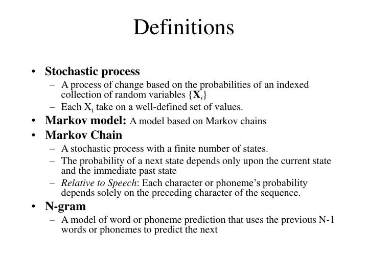
Definitions. Stochastic process A process of change based on the probabilities of an indexed collection of random variables { X i } Each X i take on a well-defined set of values. Markov model: A model based on Markov chains Markov Chain

E N D
Definitions • Stochastic process • A process of change based on the probabilities of an indexed collection of random variables {Xi} • Each Xi take on a well-defined set of values. • Markov model: A model based on Markov chains • Markov Chain • A stochastic process with a finite number of states. • The probability of a next state depends only upon the current state and the immediate past state • Relative to Speech: Each character or phoneme’s probability depends solely on the preceding character of the sequence. • N-gram • A model of word or phoneme prediction that uses the previous N-1 words or phonemes to predict the next
Hidden Markov Model • Motivation • We observe the output • We don't know what internal states the model is in • Goal: Determine the most likely internal (hidden) state • Hence the title, “Hidden” • Definition (Discrete HMM Ф = [O, S, A, B, Ω] • O = {o1, o2, …, oM} is the possible output states • S = {1, 2, …, N} possible internal HMM states • A = {aij} is the transition probability matrix from state i to j • B = {bi(k)} probability of state i outputting ok • {Ω i} = is a set of initial State Probabilities where Ωi is the probability that the system starts in state i
HMM in Computational Linguistics • Speech Recognition: • What words generated the observed acoustic signal? • Where are the word/phoneme/syllable boundaries in an acoustic signal? • Handwriting Recognition: Which words generated the observed image? • Morphology: • Which parts of speech correspond to the observed words? • Where are the word boundaries in the acoustic signal? • Which morphological word variants match the acoustic signal? • Translation: Which target language words correspond to foreign words? Demo: http://www.comp.leeds.ac.uk/roger/HiddenMarkovModels/html_dev/hmms/s3_pg1.html
Noisy Channel Model Speech Recognition • Observe: Acoustic signal (A=a1,…,an) • Challenge: Find the likely word sequence • But we also have to consider the context! • What words precede and follow the current word? • This requires knowledge of the target language
Speech Recognition Example • Observations: The digital signal features • Hidden States:The spoken word that generated the features • Simplifying Assumption: We know the acoustic signal word boundaries • Goal: Assume Word Maximizes P(Word|Observation) • Bayes Law simplifies the calculations: • P(Word|Observation) = P(Word) P(Observation|Word)/P(O) • Ignore denominator: it’s probability = 1 (we observed it after all) • Note:It is easier to compute acoustic variations in saying a word, than computing all possible acoustic observations • P(Word) can be looked up from a database • Use bi or tri grams to take the context into account • Chain rule: P(w) = P(w1)P(w2|w1)P(w3|w1,w2)P(w,w1w2…wG) • Use smoothing algorithms to insert non-zero values if needed
HMM Versus DTW • DTW employs audio fixed templates to recognize speech • DTW utilizes a fixed set of possible matching paths between spoken audio and the templates • The template with the lowest normalized distortion is most similar to the input and is selected as the recognized word • DTW algorithms can run without training (unsupervised) • HMMs advances DTW technology and employs a probabilistic model • HMM allows all possible paths, but considers their probabilities • The most likely matching word is selected as the one recognized • HMM techniques requires training of the algorithm
Natural Language HMM Assumptions • A Stochastic Markov process • System state changes are not deterministic; they vary according to some probabilistic distribution • Discrete: There is a finite system state set observable in time steps • Markov Chain: Next state depends solely on the current state • Output Assumption • Output at a given state solely depends on that state P(w1, …, wn) ≈∏i=2,n P(wi | wi-1) not P(w1, …, wn) =∏i=2,n P(wi | w1, …, wi-1) Markov Assumption Demonstration of a Stochastic Process http://cs.sou.edu/~harveyd/classes/cs415/docs/unm/movie.html
Application Example • What is the most likely word sequence?
Example • Goal: Find the probability of an observed sequence • Consider HMM describes weather and it relates to seaweed states • We have a sequence of seaweed observations. The HMM describes: All possible weather state for each observation Initial State: The probability of being in state j at initialization is that state's probability times the probability of the observation
Paths to cloudy in observation two • We can calculate the probability of reaching an intermediate state in the trellis as the sum of all possible paths to that state • The probability of it being cloudy at t = 2 is calculated from the following paths P(cloudy at t=2) = P(damp | cloudy) x P(all paths to cloudy at time t=2)
Dynamic Algorithm Next Step • We can assume that the probability of observation versus weather is always available • The probability of getting to a state through all incoming paths is also available because of the dynamic programming approach • Notice that we have an expression to calculate at time t+1 using only the partial probabilities at time t. This greatly reduces the total complexity of the calculation Demo: http://www.comp.leeds.ac.uk/roger/HiddenMarkovModels/html_dev/hmms/s3_pg1.html
An HMM Weighted Automata • Definition: • States Q = {start, ax, ix, b, aw, ae, t, dx, end} • Transition probabilities T = {.68, .20, .12, .85, .15, .16, .63, .37, .30, .54} • Non-emitting states: start and end. • The states are nodes, and the transitions are edges • The actual symbols seen are the observation sequence HMM for the word ‘about’
HMM: Trellis Model Question: How do we find the most likely sequence?
Probabilities • Forward probability: The probability of being in state si, given the partial observation o1,…,ot • Backward probability: The probability of being in state si, given the partial observation ot+1,…,oT • Transition probability:αij = P(qt = si, qt+1 = sj | observed output) The probability of being in state si at time t and going from state si, to state sj, given the complete observation o1,…,oT
Forward Probabilities αt(j) = ∑i=1,N {αt-1(i)αijbj(ot)} and αt(j) = P(O1…OT | qt = sj, λ) • Notes • λ = HMM, qt = HMM state at time t, sj = jth state, Oi = ith output • aij = probability of transitioning from state si to sj • bi(ot) = probability of observation ot resulting from si • αt(j) = probability of state j at time t given observations o1,o2,…,ot
Backward Probabilities βt(i) = ∑j=1,N {βt+1(j)αijbj(ot+1)} and βt(i) = P(Ot+1…OT | qt = si,λ) • Notes • λ = HMM, qt = HMM state at time t, sj = jth state, Oi = ith output • aij = probability of transitioning from state si to sj • bi(ot) = probability of observation ot resulting from si • βt(i) = probability of state i at time t given observations ot+1,ot+2,…,oT
The Three Basic HMM Problems Given: observation sequence O=o1,…,on and an HMM model • Problem 1 (Evaluation): What is the probability of observation O? • Problem 2 (Decoding): What state sequence best explains O? • Problem 3 (Learning): How do we adjust the HMM parameters for it to “learn” to best predict O based on the sequence of states?
Problem 1: Evaluation • Calculate observation sequence probability • Algorithm: sum probabilities of all possible state sequences that can occur in the HMM, which lead to a particular state • Naïve computation is very expensive • Given T observations and N states, there are NT possible state sequences. • If T=10 and N=5, there are 510 possible state sequences • Solution: Use dynamic programming
Forward Probabilities • Assume • λ is the automata, which is a pronunciation network for each candidate word • o1,o2,…,ot is an observation sequence of length t • Forward[t,j] = P(o1,o2,…,ot,qεQ| λ) * P(w) • This answers the question: • What is the probability that, given the partial observation sequence o1,o2,…,ot, and an HMM, λ, we arrive at state q?
1 2 3 HMM Example • O = {up, down, unchanged (Unch)} • S = {bull (1), bear (2), stable (3)} Observe 'up, up, down, down, up' What is the most likely sequence of states for this output?
Bi*Ωc = 0.7 * 0.5 0.35 0.179 0.02 0.009 0.09 0.036 t=1 t=0 Sum of α0,c * ai,c * bc Forward Probabilities X = [up, up] Note: 0.35*0.2*0.3 + 0.02*0.2*0.3 + 0.09*0.5*0.3 = 0.0357
Forward Algorithm Pseudo Code What is the likelihood of a word given an observation sequence? forward[i,j]=0 for all i,j; forward[0,0]=1.0 FOR each time step t FOR each state s FOR each state transition s to s’ forward[s’,t+1] += forward[s,t]*a(s,s’)*b[s’,ot] RETURN∑forward[s,tfinal+1] for all states s Notes • 1.a(s,s’) is the transition probability from state s to state s’ • 2.B(s’,ot) is the probability of state s’ given observation ot Complexity: O(t*|S|2) where |S| is the number of states Question: What if T=10 and N=10?
Problem 2: Decoding • Problem 1: probability of a particular observation sequence • Problem 2: most likey path through the HMM • Algorithm: similar to computing the forward probabilities • instead of summing over transitions from incoming states • compute the maximum
Viterbi Algorithm • Similar to computing the forward probabilities, but instead of summing over transitions from incoming states, compute the maximum • Forward: • Viterbi Recursion:
Bi*Ωc = 0.7 * 0.5 0.35 0.147 0.02 0.007 0.09 0.021 t=1 t=0 Maximum of α0,c * ai,c * bc Viterbi Example Observed = [up, up] State 0 State 1 State 2 Note: 0.021 = 0.35*0.2*0.3, versus 0.02*0.2*0.3 and 0.09*0.5*0.3
Viterbi Algorithm Pseudo Code What is the likelihood of a word given an observation sequence? viterbi[i,j]=0 for all i,j; viterbi[0,0]=1.0 FOR each time step t FOR each state s FOR each state transition s to s’ newScore=viterbi[s,t]*a(s,s’)*b[s’,ot] IF (newScore > viterbi[s’,t+1]) viterbi[s’,t+1] = newScore maxScore = newScore save maxScore in a queue RETURNqueue Notes • 1.a(s,s’) is the transition probability from state s to state s’ • 2.B(s’,ot) is the probability of state s’ given observation ot
Problem 3: Learning • What if we don’t know the underlying HMM? • Speech applications normally uses training data to configure the HMM (λ) • Difficulties • Setting up the parameters are difficult and/or expensive • Training data is different from the live data • Sufficient training data might not be available • We want to create a model that learns and adjusts its parameters automatically • Goal: Create λ’ from λ such that P(O| λ’) > P(O| λ) • The optimal solution to this problem is NP complete, but there are heuristics available.
Coin Flips Example • Two trick coins used to generated a sequence of heads and tails • You see only the sequence, and must determine the probability of heads for each coin Coin A Coin B
10,000 Coin Flips • Real coins • PA(heads) = 0.4 • PB(heads) = 0.8 • Initial guess • PA(heads) = 0.51 • PB(heads) = 0.49 • Learned model • PA(heads) = 0.413 • PB(heads) = 0.801 1 10 20 30 40 Conergence between iterations Iteration
Probabilities • Forward probability: The probability of being in state si, given the partial observation o1,…,ot • Backward probability: The probability of being in state si, given the partial observation ot+1,…,oT • Transition probability: The probability of being in state si at time t and going from state si, to state sj, given the complete observation o1,…,oT
Joint probabilities State i at t and j at t+1 aijbj(Xt+1)
Parameter Re-estimation • Three parameters need to be re-estimated: • The probabilities of the initial states • Transition probabilities between states: ai,j • Probabilities of output (ot) from state i: bi(ot) • The forward-backward (Baum-Welch) maximum likely estimation (MLE) is a hill climbing algorithm • Iteratively re-estimate parameters • Improves probability that an observation matches data until the algorithm converges
Expectation Maximization (EM) • The forward-backward algorithm is an instance of the more general EM algorithm • The E Step: Compute the forward and backward probabilities for a give model • The M Step: Re-estimate the model parameters • Continue until the calculations converge
Re-estimation of State Changes Forward Value Backward Value Sum forward/backward ways to arrive at time t with observed output divided by the forward/backward ways to get to state t α’ij = ∑t=1,T αi(t)αijb(ot+1) βj(t+1) Note: b(ot) is part of αi(t) ∑t=1,T αi(t)βi(t)
Re-estimating Transition Probabilities ξ(i,j) = P(state si at t and sj at t+1, emitting ot+1 given o1,…,oT and HMM λ • Recall: aij, bi(ot+1)are HMM λstate transition and state emit probabilities • Recall: αt(i) is the probability of getting to state i using observations o1,…,ot • Recall: βt(i) is the probability of getting to state i using observations oT,…,ot+1 • Note: aij*bj(ot+1)*αt(i)*βt(i) estimates the probability to transition from i to j at t • Note: Division by all possible transitions normalizes to a value between 0 and 1 Note the calculation components in the diagram on the right
- T 1 å x ( i , j ) t Where = = t 1 - T 1 å g ( i ) t = t 1 Re-estimating Transition Probabilities • The intuition behind the re-estimation equation for transition probabilities is • Formally: Note: γt(i) is the probability of being in state si at time t, given o1,o2,…oT
Re-estimating Initial State Probabilities • Initial state distribution: is the original probability that si is a start state • Re-estimated initial state distribution: • Formally: p = ˆ Probability that si is a start state at time 1 given o1,o2,…oT i
T å d g ( o , v ) ( i ) t k t = = ) t 1 T å g ( i ) t = t 1 Re-estimation of Emission Probabilities The likelihood of an output being observed from a given state • Re-estimation of Emission probabilities • Formally: Where Note that here is not related to the δin the discussion of the Viterbi algorithm!! expected number of times in state s and observe symbol o ˆ = b ( ok ) i k i expected number of times in state s i ˆ b ( ok i
Computing the New HMM Model λ’ • Original HMM λ having • Probability of transition from state i to j: ai,j • Probability of state i Emitting output ok: bi(ok) • Probability of state i being an initial state: • The Revised HMM λ’ having • Iterate until the parameters converge for all i, j, and k ˆ p = g ( i ) i 1 t 1
bull bear stable Markov Example • Problem:Model the Probability of stocks being bull, bear, or stable • Observe: up, down, unchanged • Hidden: bull, bear, stable Probability Matrix Initialization Matrix Example: What is the probability of observing up five days in a row?
Parameters for HMM states • Cepstrals • Why? They are largely statistically independent which make them suitable for classifying outputs • Delta coefficients • Why? To overcome the HMM limitation where transitions only depend on one previous state. Speech articulators change slowly, so they don’t follow the traditional HMM model. Without delta coefficients, HMM tends to jump too quickly between states • Synthesis requires more parameters than ASR • Examples: additional delta coefficients, duration and F0 modeling, acoustic energy
Training Data • Question: How do we establish the transition probability between states when that information is not available • Older Method: tedious hand marking of wave files based on spectrograms • Optimal Method: NP complete is intractable • Newer Method: HMM Baum Welsh algorithm is a popular heuristic to automate the process • Strategies • Speech Recognition: train with data from many speakers • Speech Synthesis: train with data for specific speakers
HMM limitations • HMM is a hill climbing algorithm • It finds local (not global) minimums, not global minimums • It is sensitive to initial parameter settings • HMM's have trouble modeling variable phoneme lengths • The first order Markov assumption is not quite correct • Underflows occur when multiplying probabilities. For this reason, log probabilities are normally used • HMM requires a fixed number of state changes, which doesn’t easily convert to a continuous range of values • The relationship between outputs are interrelated, not independent