Download
1 / 32
330 likes | 551 Views
Acoustic Localization by Interaural Level Difference. Rajitha Gangishetty. d. q. sound source. f. compact microphone array. Acoustic Localization. Acoustic Localization: Determining the location of a sound source by comparing the signals received by an array of microphones.

E N D
Acoustic Localization by Interaural Level Difference Rajitha Gangishetty
d q sound source f compact microphone array Acoustic Localization Acoustic Localization: Determining the location of a sound source by comparing the signals received by an array of microphones. Issues: reverberation noise Acoustic Localization by ILD
Overview • What is Interaural Level Difference (ILD)? • ILD Formulation • ILD Localization • Simulation Results • Conclusion and Future Work Acoustic Localization by ILD
Interaural time difference (ITD): relative time shift sound source microphones ILD ITD Techniques • Interaural level difference (ILD): relative energy level All previous methods (TDE, beamforming, etc.) use ITD alone. Acoustic Localization by ILD
Previous Work • Time Delay Estimation[M. S. Brandstein, H. F. Silverman, ICASSP 1997; P. Svaizer, M. Matassoni, M. Omologo, ICASSP 1997] • BeamformingJ. L. Flanagan, J.D. Johnston, R. Zahn, JASA 1985;R. Duraiswami, D. Zotkin, L.Davis, ICASSP 2001] • Accumulated Correlation[Stanley T. Birchfield, EUSIPCO 2004] • Microphone arrays [Michael S. Brandstein, Harvey F. Silverman, ICASSP 1995; P. Svaizer, M. Matassoni, M. Omologo, ICASSP 1997] • Hilbert Envelope Approach[David R. Fischell, Cecil H. Coker, ICASSP 1984] Acoustic Localization by ILD
likelihood function computed by horizontal and vertical microphone pairs contour plots of likelihood functions (overlaid and combined) microphones true location A sneak peek at the results Likelihood plots, Estimation error, Comparison of different approaches Acoustic Localization by ILD
N microphones and a source signal s(t) • Signal received by the i th microphone di = distance from source to the ithmicrophone = additive white Gaussian noise • Energy received by i th microphone ILD Formulation Acoustic Localization by ILD
For 2 mics the relation between energies and distances is • Given E1 and E2 the sound source lies on a locus of points (a circle or line) described by where, ILD Formulation Acoustic Localization by ILD
For E1 ≠ E2 the equation becomes and radius which is a circle with center In 3D the circle becomes a sphere • For E1= E2 the equation becomes which becomes a plane in 3D ILD Formulation Acoustic Localization by ILD
Isocontours for 10log(delta E) Acoustic Localization by ILD
ILD Localization Why multiple microphone pairs? • With only two microphones source is constrained to lie on a curve • The microphones cannot pinpoint the sound source location • We use multiple microphone pairs • The intersection of the curves yield the sound source location Acoustic Localization by ILD
Combined Likelihood Approach Localize sound source by computing likelihood at a number of candidate locations: • Define the energy ratio as • Then the estimate for the energy ratio at candidate locationis where is the location of the ith microphone • is treated as a Gaussian • random variable • Joint probability from multiple microphone • pairs is computed by combining the • individual log likelihoods Acoustic Localization by ILD
Hilbert Transform • The Hilbert transform returns a complex sequence, from a real data sequence. • The complex signal x = xr + i*xi has a real part, xr, which is the original data, and an imaginary part, xi, which contains the Hilbert transform. • The imaginary part is a version of the original real sequence with a 90° phase shift. • Sines are therefore transformed to cosines and vice versa. Acoustic Localization by ILD
xr[n] xr[n] Complex Signal x[n] Hilbert Transformer h[n] xi[n] -j , 0<w<pi j , -pi<w<0 where ‘w’ is the angular frequency H(ejw) = Hilbert Transformer In Frequency domain, Xi(ejw) = H(ejw)Xr(ejw) The Hilbert transformed series has the same amplitude and frequency content as the original real data and includes phase information that depends on the phase of the original data. Acoustic Localization by ILD
(0o)2 (90o) (90o)2 Hilbert Envelope Approach • All-pass filter circuit produces two signals with equal amplitude but 90 degrees out of phase. • Square root of the sum of squares is taken. Acoustic Localization by ILD
Simulated Room Acoustic Localization by ILD
Simulation Results • The algorithm • Accurately estimates the angle to the sound source in some scenarios • Exhibits bias toward far locations (unable to reliably estimate the distance to the sound source) • Is sensitive to noise and reverberation Acoustic Localization by ILD
Results of delta E Estimation • The estimation is highly dependent upon the • sound source location • amount of reverberation • amount of noise • size of the room • relative positions of source and microphones Acoustic Localization by ILD
5x5 m room, theta = 45 deg , no noise, no reverberation, d = 2m Likelihood plots Acoustic Localization by ILD
5x5 m room, theta = 90 deg , SNR = 0db, reflection coefficient = 9, d = 2m Likelihood plots Acoustic Localization by ILD
5x5 m room, theta = 0 deg , SNR = 0db, reflection coefficient = 9, d = 1m Likelihood plots Acoustic Localization by ILD
10x10 m room, theta = 0 deg , SNR = 0db, reflection coefficient = 9, d = 1m angle error = 6.5 degrees Likelihood plots Acoustic Localization by ILD
5x5 m room, theta = 36 deg , SNR = 0db, reflection coefficient = 9, d = 2m angle error = 9 degrees Likelihood plots Acoustic Localization by ILD
0.7 = solid line, blue 0.8 = dotted, red 0.9 = dashed, green 20 dB = solid line, blue 10 dB = dotted, red 0 dB = dashed, green d = 1m, only reverberation d = 2m, only reverberation d = 1m, only noise d = 2m, only noise Angle Errors in a 5x5 m room Acoustic Localization by ILD
Angle error in degrees for the 5x5 m room when the source is at a distance of 1m Angle error in degrees for the 10x10 m room when the source is at a distance of 1m Acoustic Localization by ILD
Angle error in degrees for the 5x5 m room when the source is at a distance of 2m Angle error in degrees for the 10x10 m room when the source is at a distance of 2m Acoustic Localization by ILD
20 dB 10 dB 0 dB Without Hilbert = solid line, blue Matlab Hilbert = dotted line, red Kaiser Hilbert = dashed line, green 0.7 Reflection coefficient 0.8 0.9 Comparison of errors with the Hilbert Envelope Approach in a 5x5 m room Acoustic Localization by ILD
Comparison of errors with the Hilbert Envelope Approach in a 10x10 m room 20 dB 10 dB 0 dB Without Hilbert = solid line, blue Matlab Hilbert = dotted line, red Kaiser Hilbert = dashed line, green 0.7 Reflection coefficient 0.8 0.9 Acoustic Localization by ILD
5x5 m room, theta = 18 deg , SNR = 0db, reflection coefficient = 9, d = 2m angle error = 27 degrees Likelihood plots without Hilbert Envelope Acoustic Localization by ILD
Frames approach 5x5 m room, theta = 18 deg , SNR = 0db, reflection coefficient = 9, d = 2m (left), d = 1m (right) • Signal divided into 50 frames • Frame size = 92.8ms • 50% overlap in each frame Mean error = 15 deg Std Dev = 11 deg Mean error = 7 deg Std Dev = 6 deg Acoustic Localization by ILD
Conclusion and Future Work • ILD is an important cue for acoustic localization • Preliminary results indicate potential for ILD (Algorithm yields accurate results for several configurations, even with noise and reverberation) • Future work: • Investigate issues (e.g., bias toward distant locations, sensitivity to reverberation) • Experiment in real environments • Investigate ILDs in the case of occlusion • Combine with ITD to yield more robust results Acoustic Localization by ILD
Thank You Acoustic Localization by ILD