Download
1 / 27
290 likes | 681 Views
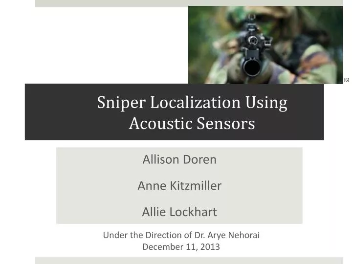
[6]. Sniper Localization Using Acoustic Sensors. Allison Doren Anne Kitzmiller Allie Lockhart. Under the Direction of Dr. Arye Nehorai December 11, 2013. Outline. Background Muzzle Blast Model Sniper Localization Maximum Likelihood Cramér-Rao Bound Mean Square Error Results

E N D
[6] Sniper Localization Using Acoustic Sensors Allison Doren Anne Kitzmiller Allie Lockhart Under the Direction of Dr. AryeNehorai December 11, 2013
Outline • Background • Muzzle Blast Model • Sniper Localization • Maximum Likelihood • Cramér-Rao Bound • Mean Square Error • Results • Detection • Conclusions
Background • Existing Work: • “Shooter Localization in Wireless Microphone Networks,” comparing muzzle blast and shock wave models and using Cramér-Rao lower bound analysis[1] • “Analysis of Sniper Localization for Mobile, Asynchronous Sensors”, relying on time difference of arrival measurements, and providing a Cramér-Rao bound for the models[2] • “ShotSpotter” uses acoustic sensors to detect outside gunshot incidents in the D.C. area[5] • Applications: • Military Operations: can be worn by soldiers or placed in vehicles • Civilian Environments: can detect gunfire to alert local authorities = sensor = shooter Example of a sensor network[2]
Types of Models • Shockwave Model (SW) • Exploits the shockwave of a gun shot, which comes about as a result of the supersonic bullets • Muzzle Blast Model (MB) • Exploits the “bang” of a gun shot • Combined Model (Shockwave and Muzzle Blast) The shockwave from the supersonic bullet reaches the microphone before the muzzle blast [1]
Muzzle Blast Model: First Step • Time of Arrival (TOA), for the ith sensor and the mth measurement: • Define Parameters: • N = total number of sensors (N = 6) • iter = number of iterations (iter = 100) • m = total number of measurements (m = 500) • i = ith sensor (i = 1, 2, …, N) • c = speed of sound (330 m/s) • = time origin of the muzzle blast (normal distribution) • = distance from the ith sensor at to the sniper position at
Muzzle Blast Model: Second Step • Muzzle Blast Time Difference of Arrival (TDOA): • Uses sensor 1 as a reference, for time synchronization purposes • = time origin of muzzle blast for ithsensor • , as defined below, where and are assumed to be independent, , and , for i= 2, 3, …, N e
Muzzle Blast Model: Second Step • Maximum Likelihood Estimation, using the conditional probability distribution p: • Maximum Likelihood (ML) and Least Squares (LS) equivalent in this simulation, because using deterministic ML method, where is the unknown parameter • Therefore, maximizing for the ML method was equivalent to minimizing the errorfor the LS method.
Cramér-Rao Bound • The Cramér-Rao Bound (CRB) is a lower bound on the variance of an unbiased estimator • We use a Multivariate Normal Distribution, because TDOA vector has a length equal to N-1
Cramér-Rao Bound • CRB for Multivariate Case • The Fisher Information Matrix (FIM) for N-variate multivariate normal distribution
Cramér-Rao Bound • In our case,
Cramér-Rao Bound • Fisher Information Matrix • For Tindependent measurements,
Mean Square Error • Compare MSE with CRB • N = number of sensors • iter = number of iterations • = our parameter • = the estimate of our parameter • Also find the MSE of our sniper position (x, y)
Signal-to-Noise Ratio (SNR) • Compare signal power to noise power • Signal Power: , where is as defined previously • Noise Power:
Results • Iterations, iter= 100 • Number of measurements (shots), m = 500 • Number of sensors, N = 6 • = 0:0.04:0.36, standard deviation of noise
Placement of sensors in Matlab model and localization error (a) Sensor network and shooter position (b) Localization error of position • Variance = 0.01 • Minimum values of error at (0,0), our true sniper location
Sensor Network Geometry Comparison of localization performance on various six sensor geometries • Shooter surrounded by sensors is ideal, but not practical • Line of sensors does not provide sufficient information
Sensor Network Geometry Comparison of localization performance on various random sensor geometries • Increased number of sensors increases accuracy, but not realistic to have this many sensors in close range
MSE of sniper position (x, y) vs. SNR MSE of position vs. SNR • As the signal-to-noise ratio increases, error decreases • Thus as noise increases, error increases
MSE of vs. SNR, with CRB r MSE of , the TDOA, vs. SNR with CRB • MSE converges to the CRB as SNR increases
Detection - general • The Neyman-Pearson Lemma [7] uses a likelihood-ratio test to choose a critical region that maximizes the power of a hypothesis test • =, false alarm • If are independent and identically distributed random samples of , and the following hypothesis test is given . • It follows that the critical region is • where k is calculated from
Detection of a shot • For this simulation, , where , where . • If • then the critical region is of the form
Detection of a shot • is rejected if and a is calculated from where . Then, and • Therefore, • will be rejected if , and will be accepted if
ROC Curve PD ROC Curve generated from detection applied in the scalar case (2 sensors) • Power, PD= • As increases, the critical region also increases, and thus power increases.
Conclusions • We used the Maximum Likelihood Method, Cramér-Rao Bound, and Mean Square Errorin the Muzzle Blast Model to analyze our simulated shooter data, with different values of variance (noise) • As predicted, MSE increases as noise increases • MSE converges to the CRB as SNR increases • We studied the concept of detection and applied it to the scalar case of detecting a sniper with two sensors • We would have liked to compare our results to actual data obtained from sensors • Further Research • Adding walls or other obstacles to sensor model • Using different types of sensors, ie. optical, infrared • Explore shockwave or combined MB-SW model • Compare results to real data
References • D. Lindgren, O. Wilsson, F. Gustafsson, and H. Habberstad, “Shooter localization in wireless sensor networks,” Information Fusion, 2009, FUSION ’09, 12th International Conference on, pp. 404-411, 2009. • G. T. Whipps, L. M. Kaplan, and R. Damarla, “Analysis of sniper localization for mobile, asynchronous sensors,” Signal Processing, Sensor Fusion, and Target Recognition XVIII, vol. 7336, 2009. • P. Bestagini, M. Compagnoni, F. Antonacci, A. Sarti, and S. Tubaro, “TDOA-based acoustic source localization in the space-range reference frame,” Multidimensional Systems and Signal Processing, Vol. March, 2013. • Stephen, Tan Kok Sin. (2006). Source localization using wireless sensor networks (Master’s thesis). Naval Postgraduate School, 2006. Web. Sept 2013. • Berkowitz, Bonnie, Emily Chow, Dan Keating and James Smallwood. “Shots heard around the District.” The Washington Post 2 Nov. 2013. Investigations Web. Nov. 2013. • Photograph of Sniper. Photograph. n.d. Shooter Localization Mobile App Pinpoints Enemy Snipers. Vanderbilt School of Engineering. Web. 11 Nov 2013. • Hogg, Robert V., and Allen T. Craig. Introduction to Mathematical Statistics. New York: Macmillan, 1978. 90-98. Print.
Thank You! • Thank you to Keyong Han, the PhD student who has been guiding us throughout this project. • Thank you to Dr. AryeNehorai for all of his help in overseeing our work and our progress.