Download
1 / 53
530 likes | 958 Views
STAT 101 Dr. Kari Lock Morgan. Normal Distribution. Chapter 5 Normal distribution Central limit theorem Normal distribution for confidence intervals Normal distribution for p-values Standard normal. Re-grade Requests. 4e potential grading mistake: 0.025 is correct

E N D
STAT 101 Dr. Kari Lock Morgan Normal Distribution • Chapter 5 • Normal distribution • Central limit theorem • Normal distribution for confidence intervals • Normal distribution for p-values • Standard normal
Re-grade Requests • 4e potential grading mistake: 0.025 is correct • Requests for a re-grade must be submitted in writing by class on Wednesday, March 5th • Partial credit will NOT be adjusted • Valid re-grade requests: • You got points off but believe your answer is correct • Points were added incorrectly • Warning: scores may go up or down
Bootstrap and Randomization Distributions Correlation: Malevolent uniforms Slope :Restaurant tips What do you notice? Mean :Body Temperatures Diff means: Finger taps Proportion : Owners/dogs Mean : Atlanta commutes
Normal Distribution • The symmetric, bell-shaped curve we have seen for almost all of our bootstrap and randomization distributions is called a normal distribution
Central Limit Theorem! For a sufficiently large sample size, the distribution of sample statistics for a mean or a proportion is normal www.lock5stat.com/StatKey
CLT for a Mean Population Distribution of Sample Data Distribution of Sample Means n = 10 n = 30 n = 50
Central Limit Theorem • The central limit theorem holds for ANY original distribution, although “sufficiently large sample size” varies • The more skewed the original distribution is (the farther from normal), the larger the sample size has to be for the CLT to work • For small samples, it is more important that the data itself is approximately normal
Central Limit Theorem • For distributions of a quantitative variable that are not very skewed and without large outliers, n ≥ 30 is usually sufficient to use the CLT • For distributions of a categorical variable, counts of at least 10 within each category is usually sufficient to use the CLT
Accuracy • The accuracy of intervals and p-values generated using simulation methods (bootstrapping and randomization) depends on the number of simulations (more simulations = more accurate) • The accuracy of intervals and p-values generated using formulas and the normal distribution depends on the sample size (larger sample size = more accurate) • If the distribution of the statistic is truly normal and you have generated many simulated randomizations, the p-values should be very close
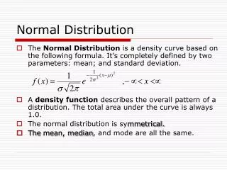
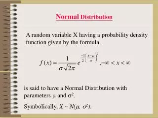
Normal Distribution • The normal distribution is fully characterized by it’s mean and standard deviation
Bootstrap Distributions If a bootstrap distribution is approximately normally distributed, we can write it as N(parameter, sd) N(statistic, sd) N(parameter, se) N(statistic, se) sd = standard deviation of variable se = standard error = standard deviation of statistic
Hearing Loss • In a random sample of 1771 Americans aged 12 to 19, 19.5% had some hearing loss (this is a dramatic increase from a decade ago!) • What proportion of Americans aged 12 to 19 have some hearing loss? Give a 95% CI. Rabin, R. “Childhood: Hearing Loss Grows Among Teenagers,” www.nytimes.com, 8/23/10.
Hearing Loss (0.177, 0.214)
Hearing Loss N(0.195, 0.0095)
Confidence Intervals If the bootstrap distribution is normal: To find a P% confidence interval , we just need to find the middle P% of the distribution N(statistic, SE)
Area under a Curve • The area under the curve of a normal distribution is equal to the proportion of the distribution falling within that range • Knowing just the mean and standard deviation of a normal distribution allows you to calculate areas in the tails and percentiles www.lock5stat.com/statkey
Hearing Loss www.lock5stat.com/statkey (0.176, 0.214)
Standardized Data • Often, we standardize the data to have mean 0 and standard deviation 1 • This is done with z-scores From x to z : From z to x: • Places everything on a common scale
Standard Normal • The standard normal distribution is the normal distribution with mean 0 and standard deviation 1
Standardized Data • Confidence Interval (bootstrap distribution): mean = sample statistic, sd = SE From z to x: (CI)
P% Confidence Interval 1. Find z-scores (–z* and z*) that capture the middle P% of the standard normal 2. Return to original scale with statistic z* SE P% -z* z*
Confidence Interval using N(0,1) If a statistic is normally distributed, we find a confidence interval for the parameter using statistic z* SE where the area between –z* and +z* in the standard normal distribution is the desired level of confidence.
Confidence Intervals Find z* for a 99% confidence interval. www.lock5stat.com/statkey z* = 2.575
z* • Why use the standard normal? • Common confidence levels: • 95%: z* = 1.96 (but 2 is close enough) • 90%: z* = 1.645 • 99%: z*= 2.576
Sin Taxes In March 2011, a random sample of 1000 US adults were asked “Do you favor or oppose ‘sin taxes’ on soda and junk food?” 320 adults responded in favor of sin taxes. Give a 99% CI for the proportion of all US adults that favor these sin taxes. From a bootstrap distribution, we find SE = 0.015
Randomization Distributions If a randomization distribution is approximately normally distributed, we can write it as N(null value, se) N(statistic, se) N(parameter, se)
p-values If the randomization distribution is normal: To calculate a p-value, we just need to find the area in the appropriate tail(s) beyond the observed statistic of the distribution
First Born Children • Are first born children actually smarter? • Explanatory variable: first born or not • Response variable: combined SAT score • Based on a sample of college students, we find • From a randomization distribution, we find SE = 37
First Born Children SE = 37 What normal distribution should we use to find the p-value? N(30.26, 37) N(37, 30.26) N(0, 37) N(0, 30.26)
First Born Children N(0, 37) www.lock5stat.com/statkey p-value = 0.207
Standardized Data • Hypothesis test (randomization distribution): mean = null value, sd = SE From x to z (test) :
p-value using N(0,1) If a statistic is normally distributed under H0, the p-value is the probability a standard normal is beyond
First Born Children SE = 37 Find the standardized test statistic Compute the p-value
z-statistic If z = –3, using = 0.05 we would (a) Reject the null (b) Not reject the null (c) Impossible to tell (d) I have no idea
z-statistic • Calculating the number of standard errors a statistic is from the null value allows us to assess extremity on a common scale
Confidence Interval Formula • IF SAMPLE SIZES ARE LARGE… From N(0,1) From original data From bootstrap distribution
Formula for p-values • IF SAMPLE SIZES ARE LARGE… From original data From H0 From randomization distribution Compare z to N(0,1) for p-value
Standard Error • Wouldn’t it be nice if we could compute the standard error without doing thousands of simulations? • We can!!! • Or at least we’ll be able to next class…
t-distribution • For quantitative data, we use a t-distributioninstead of the normal distribution • The t distribution is very similar to the standard normal, but with slightly fatter tails (to reflect the uncertainty in the sample standard deviations)
Degrees of Freedom • The t-distribution is characterized by itsdegrees of freedom (df) • Degrees of freedom are based on sample size • Single mean: df = n – 1 • Difference in means: df = min(n1, n2) – 1 • Correlation: df = n – 2 • The higher the degrees of freedom, the closer the t-distribution is to the standard normal
The Pygmalion Effect Teachers were told that certain children (chosen randomly) were expected to be intellectual “growth spurters,” based on the Harvard Test of Inflected Acquisition (a test that didn’t actually exist). These children were selected randomly. The response variable is change in IQ over the course of one year. • Source: Rosenthal, R. and Jacobsen, L. (1968). “Pygmalion in the Classroom: Teacher Expectation and Pupils’ Intellectual Development.” Holt, Rinehart and Winston, Inc.
The Pygmalion Effect Can this provide evidence that merely expecting a child to do well actually causes the child to do better? If so, how much better? SE = 1.8 *s1 and s2 were not given, so I set them to give the correct p-value