Download
1 / 1
10 likes | 212 Views
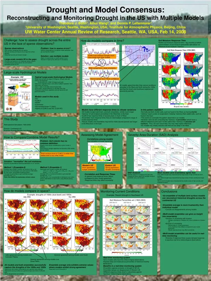
Example: VIC. Simulated Average Monthly Soil Moisture (40.25N, 112.25W), 1920-2003. Average Model Correlation. Response time (months). Drought and Model Consensus: Reconstructing and Monitoring Drought in the US with Multiple Models

E N D
Example: VIC Simulated Average Monthly Soil Moisture (40.25N, 112.25W), 1920-2003 Average Model Correlation Response time (months) Drought and Model Consensus: Reconstructing and Monitoring Drought in the US with Multiple Models Theodore J. Bohn1, Aihui Wang2, and Dennis P. Lettenmaier1 1University of Washington, Seattle, Washington, USA; 2Institute for Atmospheric Physics, Beijing, China UW Water Center Annual Review of Research, Seattle, WA, USA, Feb 14, 2008 Challenge: how to assess drought across the entire US in the face of sparse observations? How do models compare in time? How do models compare in time? • Soil Moisture Response Time • Define soil moisture response time = lag (months) at which autocorrelation of soil moisture (percentile) falls below 1/e • Measure of soil moisture “memory” Area-averaged soil moisture percentiles • Sparse observations • Soil moisture sampling sites are sparse • Remote sensing techniques only scrape the surface (literally) • Historical records are limited in length • Large-scale models fill in the gaps • A model can transform our (relatively) dense network of meteorological observations into soil moisture estimates across the US • Problem: how to assess errors? • Without observations to constrain model estimates, how can we trust the model? • Solution: use multiple models • Mean of results tends to cancel random errors • Spread of results gives estimate of uncertainty CLM3.5 soil moisture changes much more slowly than other models Wide spread here = large uncertainty Large-scale Hydrological Models • Typical Large-scale Hydrological Models • Break land surface into large (1/8-degree), flat grid cells with uniform soil properties • Continental US = 3322 1/8-degree grid cells • Most have vegetation layer, some allow multiple vegetation “tiles” • Multi-layer soil column • Input = daily or sub-daily meteorological data • Solve water, energy balances on sub-daily time step • Represent small-scale vegetation and soil dynamics with parameterizations Narrow spread here = more confidence All models agree that drier-than-normal conditions prevailed in the West and North during the 1930s and that the South and Southeast experienced several dry periods. • Models used in this study • VIC • CLM3.5 • NOAH • Catchment • Sacramento/Snow-17 (SAC) • Hybrid of CLM3.5 and VIC (CLM-VIC) • Models have different response times to climate variations • All models except Catchment, and both ensembles, exhibit much longer “memory” of soil moisture percentiles in the West than in the East • CLM3.5 has response times of several years in much of West • Ensembles have response times that are intermediate compared to range of model response times • Result: models and ensembles may tend to make dry/wet periods last longer in the West than in the East • Is this pattern realistic? • Normally we think of drier soils, such as found in the West, as having shorter “memory” due to action of evaporation (“erasing” memory) than wetter soils, such as found in the East • This seems to contradict the pattern observed in our models • However, here we are computing the “memory” of percentiles (which have a different reference point each month) rather than “memory” of absolute soil moisture. Thus, we lose seasonality; this may help explain difference • Or, models may simply assume soils that are too deep in the West This Study Retrospective Simulation: 1920-2003 Domain: Continental US Examine Average Monthly Soil Moisture Assessing Model Agreement Severity-Area-Duration (SAD) Analysis How to Compare/Combine Model Results? Correlations among models Give indication of model agreement • Problem: Soil column has no common definition • Depth of soil column considered by a given model is arbitrary • Soil moisture storage capacities and dynamics differ widely among models VIC CLM3.5 SAC CLM-VIC Driest moisture level of CLM3.5 is wetter than wettest level of any other model • Solution: “normalize” the soil moistures • Express as percentile of historical distribution (% of “normal”) • Western US • Poor agreement • Larger uncertainty • Eastern US • Strong agreement • Smaller uncertainty NOAH Catchment ENS-0 ENS-1 • Method 1 (Ensemble-0) • Express each model’s monthly soil moisture SM(y,m) as percentile of its distribution over entire period (1920-2003) for that month, using Weibull plotting position • Average the percentiles to get ensemble average percentile SMens(y,m) • Note: this method de-emphasizes extreme values • Method 2 (Ensemble-1) • Normalize each model’s monthly soil moisture • SM*(y,m) = (SM(y,m) - SMmin(m)) / (SMmax(m) - SMmin(m)) • where y = year; m = month • Average SM*(y,m) across all models to get ensemble average SMens*(y,m) • Express SMens*(y,m) as percentile of distribution over entire period (1920-2003) for that month, using Weibull plotting position • SAD Analysis • Identify regions of contiguous dry grid cells • Categorize these regions by average moisture percentile, area, and duration • Most models (and ensembles) agree that: • The 1930s drought was characterized by large areas of high severity but short duration • The 1950s drought was characterized by large areas of lower severity but longer duration • More recent droughts were characterized by smaller areas of high severity and moderate duration • Correlation and Response Times • In general, long response times (West) correspond to poor model agreement • Response times may affect uncertainty How do models compare in space? Monitoring Current Conditions Conclusions Example: droughts of 1930s (dust bowl) and 1950s Example: Recent drought in Southeast US • An ensemble of multiple land surface models can reconstruct historical droughts across the continental US • Ensemble average is more trustworthy than individual model • Cancels out disagreements among models • Multi-model ensembles can give us insight into uncertainty • Variation of uncertainty with location • Greater uncertainty in Western US, more confidence in Eastern US • Sources of uncertainty • Meteorology vs. model parameters • Long response times (West) correspond to poor model agreement • Model response times may affect uncertainty • Multi-model ensembles can be useful in real-time monitoring • Diversity of response times causes damped response to spurious real-time meteorological observations Soil Moisture Percentiles wrt (1920-2003) 2007-Nov-01 2007-Dec-01 2008-Jan-01 Ensemble-0 Little agreement among models over Colorado Plateau General agreement among models over South • Real-time monitoring system • Drive models with real-time meteorological observations • Express daily soil moistures as percentiles of historical monthly distributions General agreement among models over Great Plains • All models and both ensembles successfully capture the droughts of the 1930s and 1950s • Agreement with historic observations as to general areas affected • Agreement among models as to general shape and extent of affected area • Some disagreement as to details • Ensemble average only exhibits extreme values where models exhibit strong agreement • Especially true of Ensemble-0 • Benefits in a real-time monitoring system • Ensemble captures evolution of drought in SE US • Ensemble damps out disagreement in Western US • Different response times result in robustness against “spurious” meteorological observations