Download
1 / 53
530 likes | 664 Views
Hip Psychometrics. Peter Baldwin Joseph Bernstein Howard Wainer. Models vary in strength. When you have a lot of data, your need for a model decreases and so you can manage with a weak one. When your data are very limited, you need a strong model to lean on in order to draw inferences.

E N D
Hip Psychometrics Peter BaldwinJoseph BernsteinHoward Wainer
Models vary in strength When you have a lot of data, your need for a model decreases and so you can manage with a weak one. When your data are very limited, you need a strong model to lean on in order to draw inferences
A very strong model P(x=1| ) = exp()/[1+ exp()] 0-PL This is a strong model that requires few data to estimate its single parameter (person ability), but in return makes rigid assumptions about the data (all items must be of equal difficulty). Such a model is justified only when you don’t have enough data to reject its assumptions.
1-PL P(x=1| ) = exp(b- )/[1+ exp(b- )] This model is a little weaker and so makes fewer assumptions about the data - now items can have differential difficulty, but it assumes that all ICCs have equal slopes. If there are enough data to reject this a weaker model is usually preferred.
2-PL P(x=1| ) = exp{a(b- )}/[1+ exp{a(b- )}] This model is weaker still allowing items to have both differential difficulty and differential discriminations. But it assumes that examinees cannot get the item correct by chance.
3-PL P(x=1| ) = c + (1-c) exp{a(b- )}/[1+ exp{a(b- )}] This model is weaker still, allowing guessing, but it assumes that items are conditionally independent.
Turtles all the way down! As the amount of data we have increases, we can test the assumptions of a model and are no longer forced to use one that is unrealistic. In general we prefer the weakest model that our data will allow. Thus we often fit a sequence of models and choose the one whose fit no longer improves with more generality (further weakening).
We usually have three models In order of increasing complexity they are: • The one we fit to the data, • The one we use to think about the data, and • The one that would actually generate the data.
When data are abundant relative to the number of questions asked of them, answers can be formulated using little more than those data.
We could fit the test response data with Samejima’s polytomous IRT Model : where {ak, ck}j, k = 0, 1, ..., mj are the item category parameters that characterize the shape of the individual response functions. The aks are analogous to discriminations; the cks analogous to intercepts.
But when data are sparse, we must lean on strong models to help us draw inferences.
A study of the diagnoses of hip fractures provides a compelling illustration of the power of psychometric models to yield insights when data are sparse.
Hip fractures are common injuries; more than 250,000 annually are treated in the US alone. These fractures can be located in the shaft of the bone or in the neck of the bone connecting the shaft to the head of the femur. Femoral neck fractures vary in their severity
Garden (1961) provided a four-category classification scheme for hip fractures.
At the heart of this study are two clinical questions of interest in the diagnosis of hip fractures. • Is Garden’s approach of classifying femoral neck fractures into four categories, which is considered the de facto standard, too finely variegated to provide meaningful information given that there are only two clinical treatment choices? 2. How consistent are orthopedic surgeons in their diagnoses? Should we expect consistent judgments from individual surgeons? Are Garden’s classifications applied consistently by different surgeons?
Raw data of hip fracture diagnosis The * indicates the 2nd administration of a previously viewed radiograph
With 20 radiographs and only 12 judges how weak a model could we get away with?
We wanted to use a Bayesian version of Samejima’s polytomous model, but could we fit it with such sparse data?We decided to ask the experts.
We surveyed 42 of the world’s greatest experts in IRT, asking what would be the minimum ‘n’ required to obtain usefully accurate results.
They were almost right. Actually 12 surgeons worked just fine, so long as a few small precautions were followed. • We treated the surgeons as the items, and the radiographs as the repetitions. • We needed 165,000 iterations to get convergence .
Ethical Caveat We feel obligated to offer the warnings that: 1. These analyses were performed by professionals; inexperienced persons should not attempt to duplicate them. 2. Keep MCMC software from out of the hands of amateurs and small children.
What did we find? The model yields a stochastic description of what happens when an orthopedic surgeon meets a radiograph. As an example, consider:
Most of these results we could have gotten without the model. What does fitting a psychometric model buy us? • Standard errors - without a model all we can say is that different surgeons agree x% of the time on this radiograph. With a model we get more usable precision. • Automatic Adjustment for differential propensity for judging a fracture serious.
This is good news! On essay scoring (and the scoring of most constructed response items) the variance due to judges is usually about the same as the variance due to examinees. Surgeons do much better than ‘expert judges.’
We shall discuss the ominous ‘almost’ shortly. The variance of the radiographs is 19 times that of the variance of surgeons. We can construct an analog of reliability from this as (if we treat2x-raysas true score variance and2Doctors as error variance). Reliability = 2x-rays/(2x-rays2Doctors) These data yield an estimate of reliability of judgment equal to 0.95. Suggesting that in aggregate, on this sample of x-rays, there is almost no need for a second opinion.
The model provides us with robustness of judgment by adjusting the judgments for the differences in the propensities of the orthopedists in their tendencies to vary in severity. For example, consider case 6. Although there are three doctors who judged it a III, the other nine all placed it as a I or a II.
The model yields the probability of this case falling in each of the four categories as: I II III IV .18 .59 .21 .02 Overall, it fell solidly in the II category, and so if we had 12 different opinions on this case we would feel reasonably secure deciding to pin the fracture, for the probability of it being a I or a II was 0.77 (.18+.59).
But let’s try an experiment. Suppose we omit, for this case, all nine surgeons that scored this anything other than a III. We thus have three surgeons who all rated it a category III fracture and if we went no further the patient would have a hip replacement in his immediate future. But if we use the model, it automatically adjusts for the severity of those three judges and yields the probabilities of case 6 falling in each of the four categories as: I II III IV .03 .38 .48 .11