Download
1 / 84
880 likes | 1.16k Views
Chapter 10 Image Segmentation. 國立雲林科技大學 電子工程系 張傳育 (Chuan-Yu Chang ) 博士 Office: ES 709 TEL: 05-5342601 ext. 4337 E-mail: chuanyu@yuntech.edu.tw. Introduction. Image Segmentation Subdivides an image into its constituent regions or objects.

E N D
Chapter 10Image Segmentation 國立雲林科技大學 電子工程系 張傳育(Chuan-Yu Chang ) 博士 Office: ES 709 TEL: 05-5342601 ext. 4337 E-mail: chuanyu@yuntech.edu.tw
Introduction • Image Segmentation • Subdivides an image into its constituent regions or objects. • Segmentation should stop when the objects of interest in an application have been isolated. • Segmentation accuracy determines the eventual success or failure of computerized analysis procedures. • Image segmentation algorithm generally are based on one of two basic properties of intensity values: • Discontinuity • Partitioning an image based on abrupt changes in intensity. • Similarity • Partitioning an image into regions that are similar according to a set of predefined criteria.
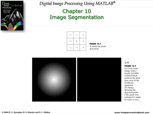
Detection of discontinuities • There are three basic types of gray-level discontinuities • Points, lines, and edges. • The most common way to look for discontinuities is to run a mask through the image in the manner described in Section 3.5. (sum of product) (10.1-1)
有小破洞 Detection of discontinuities • Point detection • An isolated point will be quit different from its surroundings. • Measures the weighted differences between the center point and its neighbors. • A point has been detected at the location on which the mask is centered ifwhere T is a nonnegative threshold. Mask計算後的結果 飛機渦輪葉片的X光影像 取(c)圖最大灰階的90%作為threshold後的結果
Detection of discontinuities • Line detection • Let R1, R2, R3, and R4 denote the response of the mask in following. • Suppose that the four masks are run individually through an image. • If, at a certain point in the image, |Ri|>|Rj|, for all j=/=i, that point is said to be more likely associated with a line in the direction of mask i. • If we are interested in detecting all the lines in an image in the direction defined by a given mask, we simply run the mask through the image and threshold the absolute value of the result. • The coefficients in each mask sum to zero.
Detection of discontinuities • We are interested in finding all the lines that are one pixel thick and are oriented at -45. • Use the last mask shown in Fig. 10.3. 偵測到的45度line 強度最強的line
Detection of discontinuities • Edge detection • An edge is a set of connected pixels that lie on the boundary between two regions. • The “thickness” of the edge is determined by the length of the ramp. • Blurred edges tend to be thick and sharp edges tend to be thin.
Detection of discontinuities • The first derivative is positive at the points of transition into and out of the ramp as we move from left to right along the profile. • It is constant for points in the ramp, • It is zero in areas of constant gray level. • The second derivative is positive at the transition associated with the dark side of the edge, negative at the transition associated wit the light side of the edge, and zero along the ramp and in areas of constant gray level. The magnitude of the first derivative can be used to detect the presence of an edge. The sign of the second derivative can be used to determine whether an edge pixel lies on the dark or light side of an edge.
Edge detection (cont.) • Two additional properties of the second derivative around an edge: • It produces two values for every edge in an image. • An imaginary straight line joining the extreme positive and negative values of the second derivative would cross zero near the midpoint of the edge. • The zero-crossing property of the second derivative is quit useful for locating the centers of thick edges.
Detection of discontinuities s=0 Image and gray-level profiles of a ramp edge • The entire transition from black to white is a single edge. First derivative image and the gray-level profile s=0.1 Second derivative image and the gray-level profile s=1 s=10
Edge detection (cont.) • The second derivative is even more sensitive to noise. • Image smoothing should be a serious consideration prior to the use of derivatives in applications . • Summaries of edge detection • To be classified as a meaningful edge point, the transition in gray level associated with that point has to be significant stronger than the background at that point. • Use a threshold to determine whether a value is “significant” or not. • We define a point in an image as being an edge point if its two dimensional first-order derivative is greater than a specified threshold. • A set of such points that are connected according to a predefined criterion of connectedness is by definition an edge. • Edge segmentation is used if the edge is short in relation to the dimensions of the image. • A key problem in segmentation is to assemble edge segmentations into longer edges. • If we elect to use the second-derivative to define the edge points in an image as the zero crossing of its second derivative.
Detection of discontinuities • Gradient operator • The gradient of an image f(x,y) at location (x,y) is defined as the vectorthe gradient vector points is the direction of maximum rate of change of f at coordinates (x,y). • The magnitude of the vector denoted ∇f, where • The direction of the gradient vector denoted by The angle is measured with respect to the x-axis.
Detection of discontinuities • Roberts cross-gradient operator • Gx=(z9-z5) • Gy=(z8-z6) • Masks of size 2x2 are awkward to implement because they do not have a clear center. • Prewitt operator • Gx=(z7+z8+z9)-(z1+z2+z3) • Gy=(z3+z6+z9)-(z1+z4+z7) • Sobel operator • Uses a weight of 2 in the center coefficient. • Gx=(z7+2z8+z9)-(z1+2z2+z3) • Gy=(z3+2z6+z9)-(z1+2z4+z7)
Detection of discontinuities • Computation of the gradient requires Gx and Gy be combined in Eq. (10.1-4), however, this implementations is not always desirable because of the computational burden required by squares and square roots. • An approach used frequently is to approximate the gradient by absolute values: • The two additional Prewitt and Sobel masks for detecting discontinuities in the diagonal directions are shown in Fig. 10.9 用來偵測對角邊界的Prewitt及Sobel mask。
Detection of discontinuities • Fig. 10.10 shows the response of the two components of the gradient, |Gx| and |Gy|. • The gradient image formed the sum of these two components.
Detection of discontinuities • Figure 10.11 shows the same sequence of images as in Fig. 10.10, but with the original image being smoothed first using a 5x5 averaging filter. • The response of each mask no shows almost no contribution due to the bricks, with the result being dominated mostly by the principal edges.
Detection of discontinuities • The horizontal and vertical Sobel masks respond about equally well to edges oriented in the minus and plus 45° direction. • If we emphasize edges along the diagonal directions, the one of the mask pairs in Fig. 10.9 should be used. • The absolute responses of the diagonal Sobel masks are shown in Fig. 10.12. • The stronger diagonal response of these masks is evident in these figures.
Detection of discontinuities • The Laplacian of a 2-D function f(x,y) is a second-order derivative defined as • For a 3x3 region, one of the two forms encountered most frequently in practice is (水平與垂直邊) • A digital approximation including the diagonal neighbors is given by (含水平、垂直、及對角邊)
Detection of discontinuities • The Laplacian generally is not used in its original form for edge detection for several reasons: • As a second-order derivative, the Laplacian typically is unacceptably sensitive noise. • The magnitude of the Laplacian produces double edges. • The Laplacian is unable to detect edge direction. • The role of the Laplacian in segmentation consists of • Using its zero-crossing property for edge location. • Using it for complementary purpose of establishing whether a pixel is on the dark or light side of an image.
Detection of discontinuities • Laplacian of a Gaussian (LoG) • The Laplacian is combined with smoothing as a precursor to finding edges via zero-crossing, consider the functionwhere r2=x2+y2 and s is the standard deviation. • Convolving this function with an image blurs the image, with the degree of blurring being determined by the value of s. • The Laplacian of h is • The function is commonly referred to as the “Laplacian of a Gaussian” (LoG), sometimes is called the ”Mexican hat” function
Detection of discontinuities • The purpose of the Gaussian function in the LoG formulation is to smooth the image, and the purpose of the Laplacian operator is to provide an image with zero crossings used to establish the location of edges.
Detection of discontinuities • Fig. 10.15(c) is a spatial Gaussian function (with a standard deviation of five pixels) used to obtain a 27x27 spatial smoothing mask. The mask was obtained by sampling this Gaussian function at equal interval. • ∇2h can be computed by application of (c) followed by (d). • The LoG result shown in Fig. 10.15(e) is the image from which zero crossings are computed to find edges. • One straightforward approach for approximating zero-crossings is to threshold the LoG image by setting all its positive values to white, and all negative values to black. • Zero-crossing occur between positive and negative values of the Laplacian. • Estimated zero-crossing, obtained by scanning the threshold image and noting the transitions between black and white.
Detection of discontinuities • Comparing Figs/ 10.15(b) and (g) • The edges in the zero-crossing image are thinner than the gradient edges. • The edges determined by zero-crossings form numbers closed loops. • “spaghetti effect” is one of the most serious drawbacks of this method. • The major drawback is the computation of zero crossing.
Edge Linking and Boundary Detection • Ideally, edge detection should yield pixels lying only on edges. • In practice, this set of pixels seldom characterizes an edge completely because of noise, breaks in the edge from nonuniform illumination, and other effects that introduce spurious intensity discontinuities. • Thus, edge detection algorithms are followed by linking procedures to assemble edge pixels into meaningful edges. • Local Processing • To analyze the characteristics of pixels in a small neighborhood about every point (x,y) in an image that has been labeled an edge point. • All points that are similar according to a set of predefined criteria are linked.
Edge Linking and Boundary Detection • The two principal properties used for establishing similarity of edge pixels: • The strength of the response of the gradient operator used to produce the edge pixel. Eq.(10.1-4) • The direction of the gradient vector. Eq. (10.1-5)
Edge Linking and Boundary Detection • An edge pixel with coordinates (x0,y0) in a predefined neighborhood of (x,y), is similar in magnitude to the pixel at (x,y) if • An edge pixel at (x0,y0) is the predefined neighborhood of (x,y)has an angle similar to the pixel at (x,y) if • A point in the predefined neighborhood of (x,y) is linked to the pixel at (x,y) if both magnitude and direction criteria are satisfied。 • This process is repeated at every location in the image. • A record must be kept of linked points as the center of the neighborhood is moved from pixel to pixel.
Edge Linking and Boundary Detection • Example 10-6: the objective is to find rectangles whose sizes makes them suitable candidates for license plates. • The formation of these rectangles can be accomplished by detecting strong horizontal and vertical edges. • Linking all points, that had a gradient value greater than 25 and whose gradient directions did not differ by more than 15°. 使用垂直的Sobel operator 分別對圖(b)及(c)進行edge linking的動作,將梯度大於25,且角度小於15度的點連起來。 使用水平的Sobel operator
Edge Linking and Boundary Detection • Global Processing via the Hough Transform • Points are linked by determining first if they lie on a curve of specified shape • Given npoints in an image, suppose that, we want to find subsets of these points that lie on straight lines. • Consider a point (xi,yi) and the general equation of a straight line in slope-intercept form, yi=axi+b. • Infinitely many lines pass through (xi,yi), but they all satisfy the equation yi=axi+b for varying values of a and b. • However, writing this equation as b=-xia+yi and considering the ab-plane yields the equation of a single line for a fixed pair (xi,yi) . • A second point (xj,yj) also has a line in parameter space associated with it, and this line intersects the lines associated with (xi,yi) at (a’, b’). • All points contained on this line have lines in parameter space that intersect at (a’, b’)
Edge Linking and Boundary Detection • Hough Transform • Subdividing the parameter space into so-called accumulator cell • Initially, these cells are set to 0. • For every point (xk, yk) in the image plane, we let the parameter a equal each of the allowed subdivisions values on the a-axis and solve for the corresponding b using the equation b=-xka+yk. • The resulting b’s are then rounded off to the nearest allowed value in the b-axis. • If a choice of ap results in solution bq,we let A(p,q)=A(p,q)+1 . • At the end of this procedure, a value of Q in A(i,j) corresponds to Q points in the xy-plane lying on the line y=aix+bj. • The number of subdivisions in the ab-plane determines the accuracy of the colinearity of these points.
Edge Linking and Boundary Detection • A problem with using the equation y=ax+b to represent a line is that the slope approaches infinity as the line approaches the vertical. • To use normal representation of a line
Edge Linking and Boundary Detection X, Y平面上五個點(1, 2, 3, 4, 5) ,在rq平面的曲線 X, Y平面上有五個點(1, 2, 3, 4, 5) 從交點A知道, 點1, 3, 5)共線。 交點B表示點2,3,4共線
Edge-linking based on Hough transform Compute the gradient of an image and thresholdit to obtain a binary image. Specify subdivisions in the rq-plane. Examine the counts of the accumulator cells for high pixel concentration. Examine the relationship between pixels in a chosen cell (依其對應的rq找出直線)。 Edge Linking and Boundary Detection
Edge Linking and Boundary Detection • Fig. (a) is an aerial infrared image containing two hangars and a runway. • Fig. (b) is a thresholded gradient image obtained using the Sobel operator. • Fig. (c) shows the Hough transform of the gradient image. • Fig. (d) shows the set of pixels linked according to the criteria • They belonged to one of the three accumulator cells with the highest count. • No gaps were longer than five pixels.
q p Edge Linking and Boundary Detection • Global Processing via Graph-Theoretic Techniques • A global approach for edge detection and linking based on representing edge segments in the form of a graph and searching the graph for low-cost paths that correspond to significant edges. • This representation provides a rugged approach that performs well in the presence of noise.。 • Graph G=(N,U) • N: set of node • U: unordered pairs of distinct elements of N • Each pair (ni,nj) of U is called arc,ni,is said to be a parent, nj is said to be a successor。 • The process of identifying the successorof a node is called expansion。 • In each graph we define levels, such that level 0 consists of a single node, called the start or root, and the nodes in the last level are called goal nodes. • Cost (ni,nj) can be associated with every arc (ni,nj) . • A sequence of nodes n1, n2,…,nk, with each node nibeing a successor of node ni-1, is called a path from n1 to nk. • The cost of the entire path is
Edge Linking and Boundary Detection Each edge elementdefined by pixels p and q,has an associated cost, defined as where His the highest gray-level valuein the image, and f(x)is the gray-levelvalue of x. 成本 座標 灰階值
Edge Linking and Boundary Detection • By convention, the point p is on the right-hand side of the direction of travel along edge elements. • To simplify, we assume that edges start in the top row and terminate in the last row. • p and q are 4-neighbors. • An arc exists between two nodes if the two corresponding edge elements taken in succession can be part of an edge. • The minimum cost path is shown dashed. • Let r(n) be an estimate of the cost of a minimum-cost path from s to n plus an estimate of the cost of that path from n to a goal node; • Here, g(n) can be chosen as the lowest-cost path from s to n found so far, and h(n) is obtained by using any variable heuristic information. (10.2-7)
Edge Linking and Boundary Detection • Graph search algorithm • Step1: Mark the start node OPEN and set g(s)=0. • Step 2: If no node is OPEN exit with failure; otherwise, continue. • Step 3: Mark CLOSE the OPEN node n whose estimate r(n) computed from Eq.(10.2-7) is smallest. • Step 4: If n is a goal node, exit with the solution path obtained by tracing back through the pointets; otherwise, continue. • Step 5: Expand node n, generating all of its successors (If there are no successors go to step 2) • Step 6: If a successor ni is not marked, set • Step 7: if a successor ni is marked CLOSED or OPEN, update its value by lettingMark OPEN those CLOSED successors whose g’ value were thus lowered and redirect to n the pointers from all nodes whose g’ values were lowered. Go to Step 2.
Edge Linking and Boundary Detection • Example 10-9: noisy chromosome silhouette and an edge found using a heuristic graph search. • The edge is shown in white, superimposed on the original image.
Thresholding • Thresholding • To select a threshold T, that separates the objects form the background. • Then any point (x,y) for which f(x,y)>T is called an object point; otherwise, the point is called a background point. • Multilevel thresholding • Classifies a point (x,y) as belonging to one object class ifT1 <f(x,y) ≤T2, and to the other object class if f(x,y) >T2 • And to the background if f(x,y)≤T2
Thresholding • In general, segmentation problems requiring multiple thresholds are best solved using region growing methods. • The thresholding may be viewed as an operation that involves tests against a function T of the formwhere f(x,y) is the gray-level of point (x,y) and p(x,y) denotes some local property of this point. • A threshold image g(x,y) is defined as • Thus, pixels labeled 1 correspond to objects, whereas pixels labeled 0 correspond to the background. • When T depends only on f(x,y) the threshold is called global. If T depends on both f(x,y) and p(x,y), the threshold is called local. • If T depends on the spatial coordinates x and y, the threshold is called dynamic or adaptive.
The role of illumination • An image f(x,y) is formed as the product of a reflectance component r(x,y) and an illumination component i(x,y). • In ideal illumination, the reflective nature of objects and background could be easily separable. • However, the image resulting from poor illumination could be quit difficult to segment. • Taking the natural logarithm of Eq.(10.3-3) (10.3-4) (10.3-5)
The role of illumination • From probability theory, • If i’(x,y) and r’(x,y) are independent random variables, the histogram of z(x,y) is given by the convolution of the histograms of i’(x,y) and r’(x,y).
The role of illumination 電腦產生的反射函數 電腦產生的照度函數 影像f(x,y)可看作是反射量r(x,y)和照度i(x,y)的乘積。 Fig. (a)*Fig(c) 物體和背景的反射特性,使她們容易被分割,但差的照明,會使產生的影像難以分割。
Thresholding • Basic global thresholding • Select an initial estimate for T • Segment the image using T • G1 : consisting of all pixels with gray level values >T • G2 : consisting of all pixels with gray level values <=T • Compute the average gray level values m1and m2 for pixels in regions G1 and G2. • Compute a new threshold value • T=0.5*(m1 + m2) • Repeat step 2 through 4 until the difference in T in successive iterations is smaller than a predefined parameter T0. • The parameter T0 is used to stop the algorithm after changes become small.
Basic Global Thresholding • To partition the image histogram by using a single global threshold T. • Segmentation is then accomplished by scanning the image pixel by pixel and labeling each pixel as object or background, depending on whether the gray level of that pixel is great or less than the value T.
Basic Global Thresholding • Fig. (a) is the original image, (b) is the image histogram. • The clear valley of the histogram. • Application of the iterative algorithm resulted in a value of 125.4 after three iterations starting with the average gray level and T0=0. • The result obtained using T=125 to segment the original image is shown in Fig. (c).
Thresholding • Basic adaptive thresholding • Imaging factors such as uneven illumination can transform a perfectly segmentable histogram into a histogram that cannot be partitioned effectively by a single global threshold. • To divide the original image into subimages and then utilize a different threshold to segment each subimage. • The key issues are • How to subdivide the image? • How to estimate the threshold for each resulting subimages? Global threshold手動將T設在山谷處。 將原始影像根據亮度的變化分成16區塊。
Thresholding 灰階值得分佈極不均勻,全域門限法注定失敗 圖10.30(c)的(1,2)及(2,2)子影像 分成更多的子影像
Thresholding • Optimal Global and Adaptive Thresholding 影像中任何像素點不是物體就是背景。 將背景誤認為物體的機率。 將物體誤認為背景的機率。 總誤差 background object